Variational Methods Applied to the Even-Parity Transport Equation

1. Variational Methods Applied to the Even-Parity Transport Equation David Sirajuddin University of Wisconsin - Madison Dept. of Nuclear Engineering and Engineering Physics NEEP 705 – Advanced Reactor Theory, Dr. Douglass L. Henderson Final Presentation December 17, 2010

2. Outline • Motivation • Development of the even-parity transport equation • Variationalconcepts • Ritz Procedure • Statement of the variational problem • 1-D slab transport • Spatial discretization • Angular treatment • Discrete Ordinates • Collision probability method • Legendre polynomial expansion • Conclusions • References Sirajuddin, David Itcanbeshown.com

3. Outline • Motivation • Development of the even-parity transport equation • Variational concepts • Ritz Procedure • Statement of the variational problem • 1-D slab transport • Spatial discretization • Angular treatment • Discrete Ordinates • Collision probability method • Legendre polynomial expansion • Conclusions • References Sirajuddin, David Itcanbeshown.com

4. Motivation • Computational methods of the raw form of the integrodifferential form of the transport equation are most readily facilitated by: • Discrete ordinates • Integral equations (e.g. collision probability methods) • These methods can become computationally expensive • Discrete ordinates • Ray-effects  many discrete ordinates must be used • Marching scheme, diamond differencing iterative solution • Integral equations • iterating on a scattering source • solving matrix equations with a full coefficient matrices • Scattering source approximation  method only accurate up to order O(D)  detrimental for large system size calculations • Computational expense may be reduced by recasting the transport equation into a variational form •  even-parity transport equation •  gives rise to a variety of approximation techniques •  solution requires solving a single matrix equation with sparse coefficient matrices Sirajuddin, David Itcanbeshown.com

5. Outline • Motivation • Development of the even-parity transport equation • Variationalconcepts • Ritz Procedure • Statement of the variational problem • 1-D slab transport • Spatial discretization • Angular treatment • Discrete Ordinates • Collision probability method • Legendre polynomial expansion • Conclusions • References Sirajuddin, David Itcanbeshown.com

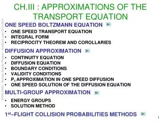
6. Development of the even-parity transport equation • Transport equation: • Boundary conditions • Define even/odd angular-parity components (even) (odd) Sirajuddin, David Itcanbeshown.com

7. Development of the even-parity transport equation • The angular flux is defined in terms of the even/odd parity fluxes where and • Scalar flux • Current Sirajuddin, David Itcanbeshown.com

8. Development of the even-parity transport equation • The even-parity equation is arrived at by considering the transport equation evaluated at W and -W • Recalling , subtracting both equations allows a relation between y- and y+  and, by definition  Calculation of the even-parity flux allows the computation of the scalar flux and the current! Sirajuddin, David Itcanbeshown.com

9. Development of the even-parity transport equation • The even-parity equation is arrived at by considering the transport equation evaluated at W and -W • Adding and subtracting the above equations produces two new equations that may be combined to eliminate y- Even-parity transport equation (isotropic scattering) Sirajuddin, David Itcanbeshown.com

10. Remarks on the even-parity transport equation • Even-parity transport equation • Even-parity  only need to solve half the angular domain • Isotropic scattering • Cannot be used directly for streaming particles in vacuum (s = 0) • Underdense materials (s small)  must check computational algorithm is stable • The equation is self-adjoint  variationalextremum principle Sirajuddin, David Itcanbeshown.com

11. Outline • Motivation • Development of the even-parity transport equation • Variationalconcepts • Ritz Procedure • Statement of the variational problem • 1-D slab transport • Spatial discretization • Angular treatment • Discrete Ordinates • Collision probability method • Legendre polynomial expansion • Conclusions • References Sirajuddin, David Itcanbeshown.com

12. Theory of Calculus of Variations • Variational methods aim to optimize functionals: • Function: , while a functional: • These functionals are often manifest as relevant integrals • Examples: minimum energy, Fermat’s principle, geodesics • Method: • Find an appropriate functional that characterizes y + • Introduce a trial function y+ + dy • Enforce dy = 0  y+ Sirajuddin, David Itcanbeshown.com

13. Theory of Calculus of Variations: Vladimirov’s functional • y+ is characterized by the even-parity transport eqn. • A relevant functional F[y+] may be computed by the inner product from the self-adjoint extension of the transport operator [2] Sirajuddin, David Itcanbeshown.com

14. Theory of Calculus of Variations: Stationary solutions • Model as • Inputting into the above functional  (after much algebra) the terms may be grouped according to • Where the zeroeth, first, and second variations depend on , (or ), and , respectively “variation” “zeroeth variation” “first variation” “second variation” Sirajuddin, David Itcanbeshown.com

15. Theory of Calculus of Variations: Stationary solutions • The first variation: • Stationary solutions, , require “first variation” Sirajuddin, David Itcanbeshown.com

16. Theory of Calculus of Variations: Stationary solutions • Examine term-by-term Sirajuddin, David Itcanbeshown.com

17. Theory of Calculus of Variations: Stationary solutions • Each term must independently vanish • Examine term-by-term Sirajuddin, David Itcanbeshown.com

18. Theory of Calculus of Variations: Stationary solutions • Examine term-by-term • Recall • Term 1 vanishes if is a solution to the even-parity transport equation. • This is called our Euler-Lagrange Equation Sirajuddin, David Itcanbeshown.com

19. Theory of Calculus of Variations: Stationary solutions • Examine term-by-term Sirajuddin, David Itcanbeshown.com

20. Theory of Calculus of Variations: Stationary solutions • Examine term-by-term • must satisfy the vacuum boundary condition Or, equivalently, , Modified natural boundary condition Sirajuddin, David Itcanbeshown.com

21. Theory of Calculus of Variations: Stationary solutions • Examine term-by-term Sirajuddin, David Itcanbeshown.com

22. Theory of Calculus of Variations: Stationary solutions • Examine term-by-term •  require no variation = 0 •  or, on the reflected surface Essential Boundary Condition Modified natural boundary condition (slab geometry) Sirajuddin, David Itcanbeshown.com

23. Outline • Motivation • Development of the even-parity transport equation • Variationalconcepts • Ritz Procedure • Statement of the variational problem • 1-D slab transport • Spatial discretization • Angular treatment • Discrete Ordinates • Collision probability method • Legendre polynomial expansion • Conclusions • References Sirajuddin, David Itcanbeshown.com

24. Solution of the variation problem: Ritz procedure • Suppose we approximate the flux: • Where are known even-parity shape functions, , and are unknown coefficients • Inputting the approximation into the functional dsafd , and enforcing  a matrix equation whose solution gives the coefficients Sirajuddin, David Itcanbeshown.com

25. Solution of the variation problem: Ritz procedure • Recasting in terms of matrices • Define ,  • Inserting into the Vladimirov functional: • where and Sirajuddin, David Itcanbeshown.com

26. Solution of the variation problem: Ritz procedure • Note that is an N x N symmetric matrix, since And • : N x 1 column vector • : 1 x N row vector • : N x N symmetric matrix • : N x N symmetrix matrix Sirajuddin, David Itcanbeshown.com

27. Solution of the variation problem: Ritz procedure • Introducing a variation in the trial function  Where , stationary solutions then imply • This general procedure is the basis for our solution strategy Sirajuddin, David Itcanbeshown.com

28. Outline • Motivation • Development of the even-parity transport equation • Variationalconcepts • Ritz Procedure • Statement of the variational problem • 1-D slab transport • Spatial discretization • Angular treatment • Discrete Ordinates • Collision probability method • Legendre polynomial expansion • Conclusions • References Sirajuddin, David Itcanbeshown.com

29. 1-D slab methods • Slab geometry: • Isotropic source distribution: S(x) • Reflective boundary at x = 0 • Vacuum boundary at x = a • The functional Then becomes Sirajuddin, David Itcanbeshown.com

30. 1-D slab methods And  Sirajuddin, David Itcanbeshown.com

31. 1-D slab methods • Translating the boundary conditions to 1-D Sirajuddin, David Itcanbeshown.com

32. Outline • Motivation • Development of the even-parity transport equation • Variationalconcepts • Ritz Procedure • Statement of the variational problem • 1-D slab transport • Spatial discretization • Angular treatment • Discrete Ordinates • Collision probability method • Legendre polynomial expansion • Conclusions • References Sirajuddin, David Itcanbeshown.com

33. 1-D methods: spatial discretization • A spatial mesh is designated • Each interval xj< x < xj+1is a finite element. To discretize, segment the independent variables according to • Where the yj approximate y(xj,m), and the hj are shape functions that span the finite the width of one finite element. i.e. [1] Sirajuddin, David Itcanbeshown.com

34. 1-D methods: spatial discretization • Linear piecewise trial functions are used for hj(x) x ≤ xj-1 xj-1 ≤ x ≤ xj xj ≤ x ≤ xj+1 xj+1 < x Sirajuddin, David Itcanbeshown.com

35. 1-D methods: spatial discretization • Inserting into the functional gives • Where Sirajuddin, David Itcanbeshown.com

36. 1-D methods: spatial discretization • Inserting into the functional gives • Where Each term involves a product of basis Recall,  only neighboring finite elements Are nonzero  A and B are N x N tridiagonal symmetric matrices Sirajuddin, David Itcanbeshown.com

37. 1-D methods: spatial discretization • Introducing a variation in the trial function into the functional • And enforcing stationary solutions gives a single matrix equation • A number of angular discretization methods may henceforth be employed to facilitate a solution Sirajuddin, David Itcanbeshown.com

38. Outline • Motivation • Development of the even-parity transport equation • Variationalconcepts • Ritz Procedure • Statement of the variational problem • 1-D slab transport • Spatial discretization • Angular treatment • Discrete Ordinates • Collision probability method • Legendre polynomial expansion • Conclusions • References Sirajuddin, David Itcanbeshown.com

39. 1-D methods: Angular discretization • The angular dependence may be handled in a number of ways • Discrete ordinates • Collision probability methods (integral equations) • Legendre polynomials Sirajuddin, David Itcanbeshown.com

40. 1-D methods: Angular discretization • The angular dependence may be handled in a number of ways • Discrete ordinates • Collision probability methods (integral equations) • Legendre polynomials Sirajuddin, David Itcanbeshown.com

41. Angular discretization: discrete ordinates • Beginning with the result of the spatial discretization • N/2 discrete ordinates are imposed • where the scalar flux may be approximated by a suitable quadrature rule • The solution may be obtained by iterating on the scattering source • The solution requires solving N/2 tridiagonal matrix equations due to evenness of the flux function, while the discrete ordinates equations require N tridiagonal matrix equation solutions at each step Sirajuddin, David Itcanbeshown.com

42. 1-D methods: Angular discretization • The angular dependence may be handled in a number of ways • Discrete ordinates • Collision probability methods (integral equations) • Legendre polynomials Sirajuddin, David Itcanbeshown.com

43. Angular discretization: integral equations • Beginning again with the result of the spatial discretization • Isolating the angular flux and integrating over angle:  Sirajuddin, David Itcanbeshown.com

44. Angular discretization: integral equations • Note the similarities • Collision probabilty method is of order D, even-parity method is order D2 • Both have nonsymmetric, dense coefficient matrices • Collision method requires analytic integration over kernels, even-parity could use quadrature rules Collision Probability Method Even-parity integral equations Sirajuddin, David Itcanbeshown.com

45. 1-D methods: Angular discretization • The angular dependence may be handled in a number of ways • Discrete ordinates • Collision probability methods (integral equations) • Legendre polynomials Sirajuddin, David Itcanbeshown.com

46. Angular discretization: legendre polynomial expansion • In addition to the spatial discretization all ready performed, the angular domain is discretized by a family of known even-parity angular basis functions (e.g. even-order Legendre polynomials) • Consider first the angular domain • Inserting this into our functional, the following is retrieved Sirajuddin, David Itcanbeshown.com

47. Angular discretization: legendre polynomial expansion • Where • i.e. the angular dependence is contained it these terms Sirajuddin, David Itcanbeshown.com

48. Angular discretization: legendre polynomial expansion • Enforcing stationary solutions with respect to a variation in the flux gives the spatial Euler-Lagrange operator • Which operates on the spatial dependence of the flux giving where Sirajuddin, David Itcanbeshown.com

49. Remarks on the even-parity transport equation • Writing out the functional shows stationary solutions of the angular flux require solving • The zeroeth moment corresponds to the scalar flux  {yj}1 = j(xj) Sirajuddin, David Itcanbeshown.com

50. Outline • Motivation • Development of the even-parity transport equation • Variationalconcepts • Ritz Procedure • Statement of the variational problem • 1-D slab transport • Spatial discretization • Angular treatment • Discrete Ordinates • Collision probability method • Legendre polynomial expansion • Conclusions • References Sirajuddin, David Itcanbeshown.com