Wouter Verkerke (NIKHEF)
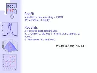
RooFit A tool kit for data modeling in ROOT (W. Verkerke, D. Kirkby ) RooStats A tool kit for statistical analysis (K. Cranmer, L. Moneta, S. Kreiss , G. Kukartsev , G. Schott, G. Petrucciani , W. Verkerke) . Wouter Verkerke (NIKHEF). Introduction.

Wouter Verkerke (NIKHEF)
E N D
Presentation Transcript
RooFitA tool kit for data modeling in ROOT(W. Verkerke, D. Kirkby)RooStatsA tool kit for statistical analysis(K. Cranmer, L. Moneta, S. Kreiss, G. Kukartsev, G. Schott,G. Petrucciani, W. Verkerke) Wouter Verkerke (NIKHEF) Wouter Verkerke, NIKHEF
Introduction • Statistical data analysis is at the heart of all (particle) physics experiments. • Techniques deployed in HEP get more and more complicated Hunting for ‘difficult signals’ (Higgs) Desire to control systematic uncertainties through simultaneous fits to control measurements • Nowadays discoveries entail simultaneous modeling of hundreds of distributions with models with over a 1000 parameters Well beyond ROOTs ‘TF1’ function classes Wouter Verkerke, NIKHEF
A structured approach to computational statistical analysis • A structured approach is needed to be able to describe and use data models needed for modern HEP analyses • 1 - Data modeling: construct a model f(x|θ) • 2 - Statistical inference on θ, given x0 and f(x|θ) • Parameter estimation ‘θ’ & variance estimation (V(θ)) MINUIT • Confidence intervals: [θ-, θ+], θ<X at 95% C.L.hypothesis testing etc: p(data|θ=0) = 1.10-7 ‘xobs’ ‘f(x|θ)’ L(θ)=f(xobs|θ) • RooFit (since 1999) • RooFit::HistFactory (since 2010) RooStats (since 2007) Wouter Verkerke, NIKHEF
RooFit – a toolkit to formulate probability models in C++ • Key concept: represent individual elements of a mathematical model by separate C++ objects Mathematical concept RooFit class variable RooRealVar function RooAbsReal PDF RooAbsPdf space point RooArgSet integral RooRealIntegral list of space points RooAbsData Wouter Verkerke, NIKHEF
RooFit core design philosophy • Functions objects are always ‘trees’ of objects, with pointers (managed through proxies) expressing relations Gauss(x,μ,σ) Math RooGaussian g RooFit diagram RooRealVar x RooRealVarm RooRealVars RooFit code RooRealVarx(“x”,”x”,-10,10) ; RooRealVarm(“m”,”y”,0,-10,10) ; RooRealVars(“s”,”z”,3,0.1,10) ; RooGaussiang(“g”,”g”,x,m,s) ;
RooFit: complete model functionality, e.g. sampling (un)binned data Example: generate 10000 events from Gaussian p.d.f and show distribution // Generate an unbinned toy MC set RooDataSet* data = gauss.generate(x,10000) ; // Generate an binned toy MC set RooDataHist* data = gauss.generateBinned(x,10000) ; // Plot PDF RooPlot* xframe = x.frame() ; data->plotOn(xframe) ; xframe->Draw() ; Can generate both binned andunbinned datasets
RooFit model functionality – max.likelihood parameter estimation // ML fit of gauss to data w::gauss.fitTo(*data) ;(MINUIT printout omitted)// Parameters if gauss now// reflect fitted valuesmean.Print() ;sigma.Print() ;RooRealVar::mean = 0.0172335 +/- 0.0299542 RooRealVar::sigma = 2.98094 +/- 0.0217306 // Plot fitted PDF and toy data overlaid RooPlot* xframe= x.frame() ; data->plotOn(xframe) ; gauss.plotOn(xframe) ; PDFautomaticallynormalizedto dataset
RooFit implements normalized probability models • Normalized probability (density) models are the basis of all fundamental statistical techniques • Defining feature: • Normalization guarantee introduces extra complication in calculation, but has important advantages • Directly usable in fundamental statistical techniques • Easier construction of complex models (will shows this in moment) • RooFit provides built-in support for normalization, taking away down-side for users, leaving upside • Default normalization strategy relies on numeric techniques, but user can specify known (partial) analytical integrals in pdf classes. Wouter Verkerke, NIKHEF
The power of conditional probability modeling • Take following model f(x,y): what is the analytical form? • Trivially constructed with(conditional) probabilitydensity functions! Gauss f(x|a*y+b,1) Gauss g(y,0,3) F(x,y) = f(x|y)*g(y) Wouter Verkerke, NIKHEF
Coding a conditional product model in RooFit • Construct each ingredient with a single line of code Gauss f(x,a*y+b,1) RooRealVar x(“x”,”x”,-10,10) ; RooRealVar y(“y”,”y”,-10,10) ; RooRealVar a(“a”,”a”,0) ; RooRealVar b(“b”,”b”,-1.5) ; RooFormulaVar m(“a*y+b”,a,y,b) ; RooGaussian f(“f”,”f”,x,m,C(1)) ; RooGaussian g(“g”,”g”,y,C(0),C(3)) ; RooProdPdf F(“F”,”F”,g,Conditional(f,y)) ; Gauss g(y,0,3) F(x,y) = f(x|y)*g(y) Note that code doesn’t care if input expression is variable or function! Wouter Verkerke, NIKHEF
Building power – most needed shapes already provided • RooFit provides a collection of compiled standard PDF classes RooBMixDecay Physics inspired ARGUS,Crystal Ball, Breit-Wigner, Voigtian,B/D-Decay,…. RooPolynomial RooHistPdf Non-parametric Histogram, Kernel estimation RooArgusBG RooGaussian Basic Gaussian, Exponential, Polynomial,…Chebychev polynomial Easy to extend the library: each p.d.f. is a separate C++ class
Individual classes can encapsulate powerful algorithms • Example: a ‘kernel estimation probability model’ • Construct smooth pdf from unbinned data, using kernel estimation technique • Example • Alsoavailableforn-D data Adaptive Kernel:width of Gaussian depends on local event density Summed pdf for all events Gaussian pdffor each event Sample of events w.import(myData,Rename(“myData”)) ; w.factory(“KeysPdf::k(x,myData)”) ;
Advanced modeling building – template morphing • At LHC shapes are often derived from histograms, instead of relying on analytical shapes . Construct parametric from histograms using ‘template morphing’ techniques Parametric model: f(x|α) Inputhistogramsfrom simulation
Code example – template morphing • Example of template morphingsystematic in a binnedlikelihood Class from the HistFactory project(K. Cranmer, A. Shibata, G. Lewis, L. Moneta, W. Verkerke) // Construct template models from histograms w.factory(“HistFunc::s_0(x[80,100],hs_0)”) ; w.factory(“HistFunc::s_p(x,hs_p)”) ; w.factory(“HistFunc::s_m(x,hs_m)”) ; // Construct morphing model w.factory(“PiecewiseInterpolation::sig(s_0,s_,m,s_p,alpha[-5,5])”) ; // Construct full model w.factory(“PROD::model(ASUM(sig,bkg,f[0,1]),Gaussian(0,alpha,1))”) ; Wouter Verkerke, NIKHEF
Advanced model building – describe MC statistical uncertainty • Histogram-based models have intrinsic uncertainty to MC statistics… • How to express corresponding shape uncertainty with model params? • Assign parameter to each histogram bin, introduce Poisson ‘constraint’ on each bin • ‘Beeston-Barlow’ technique. Mathematically accurate, but introduce results in complex models with many parameters. Binned likelihood with rigid template Subsidiary measurementsof s ,b from s~,b~ Response functionw.r.t. s, b as parameters Normalized NP model (nominal value of all γ is 1)
Code example – Beeston-Barlow • Beeston-Barlow-(lite) modelingof MC statisticaluncertainties // Import template histogram in workspace w.import(hs) ; // Construct parametric template models from histograms// implicitly creates vector of gamma parameters w.factory(“ParamHistFunc::s(hs)”) ; // Product of subsidiary measurement w.factory(“HistConstraint::subs(s)”) ; // Construct full model w.factory(“PROD::model(s,subs)”) ; Wouter Verkerke, NIKHEF
Code example: BB + morphing • Template morphing modelwith Beeston-Barlow-liteMC statistical uncertainties // Construct parametric template morphing signal model w.factory(“ParamHistFunc::s_p(hs_p)”) ; w.factory(“HistFunc::s_m(x,hs_m)”) ; w.factory(“HistFunc::s_0(x[80,100],hs_0)”) ; w.factory(“PiecewiseInterpolation::sig(s_0,s_,m,s_p,alpha[-5,5])”) ; // Construct parametric background model (sharing gamma’s with s_p) w.factory(“ParamHistFunc::bkg(hb,s_p)”) ; // Construct full model with BB-lite MC stats modeling w.factory(“PROD::model(ASUM(sig,bkg,f[0,1]),HistConstraint({s_0,bkg}),Gaussian(0,alpha,1))”) ;
From simple to realistic models: composition techniques • Realistic models with signal and bkg, and with control regions built from basic shapes using addition, product, convolution, simultaneousoperator classes SUM PROD CONV SIMUL + * = = = =
Graphical example of realistic complex models variables function objects Expression graphs areautogenerated using pdf->graphVizTree(“file.dot”)
Abstracting model building from model use - 1 • For universal statistical analysis tools (RooStats), must be have universal functionality of models (independent of structure and complexity) • Was already possible in RooFit since 1999 Fitting Generating data = model.generate(x,1000) RooAbsPdf model.fitTo(data) RooDataSet RooAbsData Wouter Verkerke, NIKHEF
Abstracting model building from model use - 2 • Must be able to practicallyseparate model building code from statistical analysis code. • Solution: you can persist RooFit models of arbitrary complexity in ‘workspace’ containers • The workspace concept has revolutionized the way people share and combine analyses! Realizes complete and practicalfactorization of process of building and using likelihood functions! RooWorkspace w(“w”) ; w.import(sum) ; w.writeToFile(“model.root”) ; model.root RooWorkspace Wouter Verkerke, NIKHEF
Using a workspace file given to you… // Resurrect model and data TFile f(“model.root”) ; RooWorkspace* w = f.Get(“w”) ; RooAbsPdf* model = w->pdf(“sum”) ; RooAbsData* data = w->data(“xxx”) ; // Use model and data model->fitTo(*data) ; RooPlot* frame = w->var(“dt”)->frame() ; data->plotOn(frame) ; model->plotOn(frame) ; RooWorkspace Wouter Verkerke, NIKHEF Wouter Verkerke, NIKHEF
Persistence of really complex models works too! Atlas Higgs combination model (23.000 functions, 1600 parameters) F(x,p) x p Model has ~23.000 function objects, ~1600 parameters Reading/writing of full model takes ~4 secondsROOT file with workspace is ~6 Mb
An excursion – Collaborative analyses with workspaces • Workspaces allow to share and modify very complex analyses with very little technical knowledge required • Example: Higgs coupling fits Confidenceintervalson Higgsfermion,bosoncouplings Full Higgs model Signalstrengthin 5channels Reparametrizein terms of fermion,bosonscale factors Wouter Verkerke, NIKHEF
An excursion – Collaborative analyses with workspaces • How can you reparametrize existing Higgs likelihoods in practice? • Write functions expressions corresponding to new parameterization • Edit existing model RooFormulaVarmu_gg_func(“mu_gg_func”,“(KF2*Kg2)/(0.75*KF2+0.25*KV2)”, KF2,Kg2,KV2) ; w.import(mu_gg_func) ; w.factory(“EDIT::newmodel(model,mu_gg=mu_gg_gunc)”) ; Top node of modifiedHiggs combination pdf Modification prescription:replace parameter mu_ggwith function mu_gg_funceverywhere Top node of originalHiggs combination pdf Wouter Verkerke, NIKHEF
RooStats – Statistical analysis of RooFit models • With RooFits one has (almost) limitless possibility to construct probability density models • With the workspaces one also has the ability to deliver such models to statistical tools that are completely decoupled from the model construction code. Will now focus on the design of those statistical tools • The RooStats projected was started in 2007 as a joint venture between ATLAS, CMS, the ROOT team and myself. Goal: to deliver a series of tools that can calculate intervals and perform hypothesis tests using a variety of statistical techniques • Frequentist methods (confidence intervals, hypothesis testing) • Bayesian methods (credible intervals, odd-ratios) • Likelihood-based methods Confidence intervals: [θ-, θ+],or θ<X at 95% C.L.Hypothesis testing: p(data|θ=0) = 1.10-7 Wouter Verkerke, NIKHEF
RooStats class structure Wouter Verkerke, NIKHEF
RooStats class structure Abstract interface for procedureto calculate a confidence intervalAbstract interface for result“[θ-, θ+]at 68% C.L”.“θ<X at 95% C.L.” Multiple concrete implementations for calculators and corresponding result containers (reflecting various statistical techniques) Wouter Verkerke, NIKHEF
RooStats class structure Abstract interface for hypothesis tester to calculate a p-valueConcrete result class“pθ=0=1.1 10-7” Multiple concrete implementations for calculators, corresponding to various statistical techniques to calculate p-value Wouter Verkerke, NIKHEF
RooStats class structure Concepts of interval calculationand hypothesis testing are linkedfor certain (frequentist) statistical methods. Also has abstract interface for ‘combined calculators’ thatcan perform both types of calculations Wouter Verkerke, NIKHEF
Working with RooStats calculators • Calculators interface to RooFit via a ‘ModelConfig’ object • ModelConfigcompletes f(x|θ) from workspace with additional information to become an unambiguous statistical problem specification (together with xobs) • E.g. which of parameters θare ‘of interest’ which are ‘nuisance parameters’. • For certain types of complex models, additional info is needed • Calculator works for any model, no matter how complex Wouter Verkerke, NIKHEF
Some famous RooFit/RooStats results RooFit workspace with Atlas Higgs combination model (23.000 functions, 1600 parameters) RooStats hypothesis testing(p-value of bkg hypothesis) RooStats interval calculation(upper limit intervals at 95%)
Performance considerations • While functionality is (nearly) universal, good computational performance for all models requires substantial work behind the scenes. • Will highlight three techniques that are used to boost performance • Heuristic constant-expression detection • Identify (highest)-level constant expression in user expression in a given use context and prevent unnecessary recalculation of these • (Pseudo)-vectorization • Reorder calculations to approach concept of vectorization • Parallelization • Exploit pervasive ability of CPU farms and multi-core host to parallelize calculations that intrinsically of a repetitive nature • The boundary condition of all optimizations is that user code should not need to accommodate these. • User probability models are often already complex, must be kept in ‘most readable’ representation • Use RooFit model introspection to reorganize user functions ‘on the fly’ in vectorization-friendly order Wouter Verkerke, NIKHEF
Optimization of likelihood calculations • Likelihood evaluates pdf at all data points, essentially a ‘loop’ call As written by user, the p.d.f is a scalar expression that is unaware of underlyingrepeated calculation of likelihood Wouter Verkerke, NIKHEF
Level-1 optimization of likelihood calculation • RooFit can heuristically detect constant terms (depends only on observables, not on parameters) are pre-calculated, cached with likelihood dataset. Calculation tree modified to omit recalculation of g Wouter Verkerke, NIKHEF
Level-2 optimization of likelihood calculation • Can also apply caching strategy to all functions nodes, instead of just constant nodes Depends on m Depends on a,b To ensure correct calculation: Value cache of non-constant function objectswill be invalidated if dependent parameterschanged Faster than level-1 if non-constant cachemiss rate <100% Wouter Verkerke, NIKHEF
What is the value cache miss rate for non-constant objects? • It is quite a bit better than 100% as most MINUIT calls to likelihood vary one parameter at a time (to calculate derivative) Computed cached values will often stay valid prevFCN = 5170.289989 FCN=5170.53 FROM MIGRAD STATUS=INITIATE 6 CALLS 7 TOTAL prevFCN = 4495.931306 a=0.9961, b=0.106, c=0.06274, prevFCN = 3936.921265 a=0.9967, prevFCN = 3936.938281 a=0.9954, prevFCN = 3936.907905 a=0.9965, prevFCN = 3936.933086 a=0.9956, prevFCN = 3936.911321 a=0.9961, b=0.108, prevFCN = 3937.05644 b=0.104, prevFCN = 3936.790003 b=0.1074, prevFCN = 3937.014478 b=0.1046, prevFCN = 3936.829929 b=0.106, c=0.06845, prevFCN = 3936.934463 c=0.05703, prevFCN = 3936.911648 c=0.06688, prevFCN = 3936.930463 c=0.05861, prevFCN = 3936.913944 a=1, b=-0.02103, c=0.02074, prevFCN = 3936.613348 a=0.9982, b=0.04018, c=0.04096, Only a changes, cachesdepending on b,c remain valid Only b changes, cachesdepending on a,c remain valid Only c changes, cachesdepending on b,c remain valid
From level-2 optimization to vectorization • Note that resequencing of calculation in full level-2 optimization mode results in ‘natural ordering’ for complete vectorization Level-1 sequence Level-2-max sequence m(y0) f(m0) g(x0) Model(f0,g0) m(y0) m(y1) m(y2) f(m0) f(m1) f(m2) g(x0) g(x1) g(x2) Model(f0,g0) Model(f1,g1) Model(f2,g2) m(y1) f(m1) g(x1) Model(f1,g1) m(y2) f(m2) g(x2) Model(f2,g2) Wouter Verkerke, NIKHEF
Work in progress – automatic code vectorization • Axel noted in his plenary presentation that ‘vectorization’ is invasive… True, but modular structure of RooFit function expression allows this invasive reorganization to be performed automatically. Aim to vectorize code without making the ‘user code’ messy! Construct custom sequence driver on the fly with CLING to eliminate virtual function calls Vectorized sequencing Level-2 optimizationensures all inputs are already in vector form But, as inputsare already always held in proxies in user code, user code is unaware of scalar/vector nature of inputs
Other parallelization techniques – multicore Likelihood calculation • Parallelization of calculations already introduce at a higher level • Multi-core calculation of likelihood at the granularity of the event level, rather than the function call level • Trivial use invocation make this already popular with users • But load balancing can become uneven for ‘simultaneous fits’ (not every event has the same probability model in that case) MultiCore parallelization m(y0) f(m0) g(x0) Model(f0,g0) m(y1) f(m1) g(x1) Model(f1,g1) m(y2) f(m2) g(x2) Model(f2,g2) model->fitTo(data,NumCPU(8),…) Wouter Verkerke, NIKHEF
Parallelization using PROOF • Simple parallelization of likelihood calculation using NumCPU(n) option of RooAbsPdf::fitTo() very popular, but restricted to likelihood calculations • Another common CPU-intensive task are toy studies • Have generic interface to PROOF(-lite) to parallelize loop tasks.Also used by RooStats for sampling procedures Accumulate fit statistics Input model Generate toy MC Fit model Distribution of - parameter values - parameter errors - parameter pulls Repeat N times Wouter Verkerke, NIKHEF
Summary • RooFit and RooStats allow you to perform advanced statistical data analysis • LHC Higgs results a prominent example • RooFit provides (almost) limitless model building facilities • Concept of persistable model workspace allows to separate model building and model interpretation • HistFactory package introduces structured model building for binned likelihood template models that are common in LHC analyses • RooStats provide a wide set of statistical tests that can be performed on RooFit models • Bayesian, Frequentist and Likelihood-based test concepts • Wide range op options (Frequentist test statistics, Bayesian integration methods, asympotic calculators…) Wouter Verkerke, NIKHEF