Download
1 / 47
470 likes | 619 Vues
CSCE 580 Artificial Intelligence Ch.3 [P]: States and Searching. Fall 2012 Marco Valtorta mgv@cse.sc.edu. Acknowledgment. The slides are based on the textbook [P] and other sources, including other fine textbooks [AIMA-2] and [AIMA-3]

E N D
CSCE 580Artificial IntelligenceCh.3 [P]: States and Searching Fall 2012 Marco Valtorta mgv@cse.sc.edu
Acknowledgment • The slides are based on the textbook [P] and other sources, including other fine textbooks • [AIMA-2] and [AIMA-3] • David Poole, Alan Mackworth, and Randy Goebel. Computational Intelligence: A Logical Approach. Oxford, 1998 • David Poole and Alan Mackworth. Artificial Intelligence: Foundations of Computational Agents. Cambridge, 2010 [P] • Ivan Bratko. Prolog Programming for Artificial Intelligence, Third Edition. Addison-Wesley, 2001 • George F. Luger. Artificial Intelligence: Structures and Strategies for Complex Problem Solving, Sixth Edition. Addison-Welsey, 2009
Searching • Often we are not given an algorithm to solve a problem, but only a specification of what is a solution---we have to search for a solution • A typical problem is when the agent is in one state, it has a set of deterministic actions it can carry out, and wants to get to a goal state • Many AI problems can be abstracted into the problem of finding a path in a directed graph • Often there is more than one way to represent a problem as a graph
Directed Graphs • A graph consists of a set N of nodes and a set A of ordered pairs of nodes, called arcs • Node n2 is a neighbor of n1 if there is an arc from n1 to n2, that is, if (n1, n2) A. More commonly, we say that n2 is a successor of n1. • A path is a sequence of nodes (n0, n1,. . ., nk) such that (ni, ni+1) A. (Sometimes, a path is defined as a sequence of arcs.) • Given a set of start nodes and goal nodes, a solution is a path from a start node to a goal node • Often there is a cost associated with arcs and the cost of a path is the sum of the costs of the arcs in the path
Example Problem for Delivery Robot The robot wants to get from outside room 103 to the inside of room 123 Names (such as r101) labels interesting locations Bold labels (such as mail) will be used to illustrate search
Partial Search Space for a Video Game Grid game: collect coins C1, C2, C3, C4, don't run out of fuel, and end up at location (1, 1)
Graph Searching • Generic search algorithm: given a graph, start nodes, and goal nodes, incrementally explore paths from the start nodes • Maintain a frontier of paths from the start node that have been explored • As search proceeds, the frontier expands into the unexplored nodes until a goal node is encountered • The way in which the frontier is expanded defines the search strategy
Graph Search Algorithm • More solution paths may be returned by continuing after line 15 • Which value is selected from the frontier at each stage defines the search strategy • The neighbors defines the graph. • goal defines what is a solution • If the path chosen does not end at a goal node and the node at the end has no neighbors, extending the path means removing the path
Depth-first Search • Depth-first search treats the frontier as a stack • It always selects one of the last elements added to the frontier. • If the list of paths on the frontier is [p1, p2, . . .] • p1 is selected. Paths that extend p1 are added to the front of the stack (in front of p2) • p2 is only selected when all paths from p1 have been explored.
Complexity of Depth-first Search • Depth-first search isn't guaranteed to halt on infinite graphs or on graphs with cycles, even if the goal node is at finite distance from the start node • The space complexity is linear in the size of the path being explored • Search is unconstrained by the goal until it happens to stumble on the goal
Breadth-first Search • Breadth-first search treats the frontier as a queue. • It always selects one of the earliest elements added to the frontier • If the list of paths on the frontier is [p1, p2, . . ., pr] • p1 is selected. Its neighbors are added to the end of the queue, after pr • p2 is selected next
Complexity of Breadth-first Search • The branching factor of a node is the number of its neighbors • If the branching factor for all nodes is finite, breadth-first search is guaranteed to find a solution if one exists • It is guaranteed to find the path with fewest arcs • Time complexity is exponential in the path length: bn, where b is branching factor, n is path length • The space complexity is exponential in path length: bn • Search is unconstrained by the goal
Lowest-cost-first search (Dijkstra’s algorithm) • Sometimes there are costs associated with arcs. The cost of a path is the sum of the costs of its arcs • At each stage, lowest-cost-first search selects a path on the frontier with lowest cost • The frontier is a priority queue ordered by path cost • It finds a least-cost path to a goal node • When arc costs are equal, it is identical to breadth-first search, except for the stopping condition
Heuristic Search • Idea: don't ignore the goal when selecting paths • Often there is extra knowledge that can be used to guide the search: heuristics • h(n) is an estimate of the cost of the shortest path from node n to a goal node • h(n) uses only readily obtainable information (that is easy to compute) about a node • h can be extended to paths: h(<n0, . . ., nk>) = h(nk) • h(n) is an underestimate if there is no path from n to a goal that has path cost less than h(n) • i.e., h(n) is a lower bound of the cost of the shortest path to n, f*(n) = h*(n)
Example Heuristic Functions • If the nodes are points on a Euclidean plane and the cost is the distance, we can use the straight-line distance from n to the closest goal as the value of h(n) • If the nodes are locations and cost is time, we can use the distance to a goal divided by the maximum speed • If the goal is to collect all of the coins and not run out of fuel, the cost is an estimate of how many steps it will take to collect the rest of the coins, refuel when necessary, and return to goal position
Best-first Search • Idea: select the path whose end is closest to a goal according to the heuristic function. • Best-first search selects a path on the frontier with minimal h-value • It treats the frontier as a priority queue ordered by h
Complexity of Best-first Search • It uses space exponential in path length • It isn't guaranteed to find a solution, even if one exists • It doesn't always find the shortest path
A* Search • A* search uses both path cost and heuristic values • cost(p) is the cost of the path p • h(p) estimates of the cost from the end of p to a goal • f (p) = cost(p) + h(p) • f (p) estimates of the the total path cost of going from a start node to a goal via p
A* Search Algorithm • A is a mix of lowest-cost-first and best-first search • It treats the frontier as a priority queue ordered by f (p) • It always selects the node on the frontier with the lowest estimated distance from the start to a goal node constrained to go via that node
Admissibility of A* • If there is a solution, A always finds an optimal solution (the first path to a goal selected) if • the branching factor is finite • arc costs are bounded above zero (there is some epsilon > 0 such that all of the arc costs are greater than epsilon), and • h(n) is an underestimate of the cost of the shortest path from n to a goal node
Why is A* admissible? Proof Sketch • If a path p to a goal is selected from a frontier, can there be a shorter path to a goal? • Suppose path p’ is on the frontier. Because p was chosen before p’, and h(p) = 0: Because h is an underestimate: • for any path p’’ to a goal that extends p’ • So cost(p) ≤ cost(p”) for any other path p” to a goal • There is always an element of an optimal solution path on the frontier before a goal has been selected • A* halts because the costs of the paths on the frontier keeps increasing and will eventually exceed any finite number
Admissibility of A*: Proof Proposition 3.1 [P]. (A* admissibility): If there is a solution, A* always finds a solution, and the first solution found is an optimal solution, if the branching factor is finite (each node has only a finite number of neighbors), arc costs are greater than some e > 0, and h(n) is a lower bound on the actual minimum cost of the lowest cost path from n to a goal node. Proof. Part A: A solution will be found. If the arc costs are all greater than some e > 0, eventually for all paths p in the frontier, cost(p) will exceed any finite number, and thus will exceed a solution cost if there is one (at depth in the search tree no greater than m/e, where m is the solution cost). As the branching factor is finite, there is only a finite number of nodes that need to be expanded before the search tree could get this size, but the A* search would have found a solution by then. Part B: The first path to a goal selected is an optimal path. The f-value for any node on an optimal solution path is less than or equal to the f-value of an optimal solution. This is because h is an underestimate of the actual cost from a node to a goal. Thus the f-value of a node on an optimal solution path is less than the f-value for any non-optimal solution. Thus a non-optimal solution can never be chosen while there is a node on the frontier that leads to an optimal solution (as an element with minimum f-value is chosen at each step). So, before it can select a non-optimal solution, it will have to pick all of the nodes on an optimal path, including each of the optimal solutions.
Admissibility of A* • See Section 3.1.3 of: Judea Pearl. Heuristics: Intelligent Search Strategies for Computer Problem Solving. Addison-Wesley, 1984. • Especially Lemma 1 and Theorem 2 (pp. 77-78) • Note that admissibility of A* does not require monotonicity of the heuristics. [AIMA] claims otherwise on p.99. The confusion is probably due to the fact that admissibility only requires an optimal solution to be returned for a goal node (for which h=0), rather than for every node that is CLOSED • A* finds shortest paths to every node it closes with monotone (consistent) heuristics
Cycle Checking • A searcher can prune a path that ends in a node already onvthe path, without removing an optimal solution. • Using depth-first methods, with the graph explicitly stored, this can be done in constant time. • For other methods, the cost is linear in path length.
Multiple-Path Pruning • Multiple path pruning: prune a path to node n that the searcher has already found a path to • Multiple-path pruning subsumes a cycle check • This entails storing all nodes it has found paths to • Want to guarantee that an optimal solution can still be found
Multiple-Path Pruning and Optimal Solutions • Problem: what if a subsequent path to n is shorter than the first path to n? • remove all paths from the frontier that use the longer path. • change the initial segment of the paths on the frontier to use the shorter path • ensure this doesn't happen. Make sure that the shortest path to a node is found first • True for the lowest-cost algorithm (Dijkstra’s algorithm) • Not true in general for A*, but true for A* with monotone (consistent) heuristics
Multiple-Path Pruning and A* • Suppose path p to n was selected, but there is a shorter path to n. Suppose this shorter path is via path p’ on the frontier. • Suppose path p’ ends at node n’ • cost(p) + h(n) <= cost(p’) + h(n’) because p was selected before p’ • cost(p’) + cost(n’, n) < cost(p) because the path to n via p’ is shorter cost(n’, n) < cost(p) - cost(p’) <= h(n’) - h(n): • You can ensure this doesn't occur if • |h(n’) - h(n)| < cost(n’, n) • Such a heuristic is said to be consistent
Monotone Restriction • Heuristic function h satisfies the monotone restriction if |h(m) - h(n)| <= cost(m, n) for every arc <m,n> • If h satises the monotone restriction, A* with multiple path pruning always finds the shortest path to a goal
Iterative Deepening • So far all search strategies that are guaranteed to halt use exponential space • Idea: let's recompute elements of the frontier rather than saving them • Look for paths of depth 0, then 1, then 2, then 3, etc • You need a depth-bounded depth-first searcher • If a path cannot be found at depth B, look for a path at depth B + 1. Increase the depth-bound when the search fails unnaturally (depth-bound was reached)
Iterative Deepening Complexity Complexity with solution at depth k and branching factor b:
Depth-first Branch-and-Bound • Way to combine depth-first search with heuristic information • Finds optimal solution • Most useful when there are multiple solutions, and we want an optimal one • Uses the space of depth-first search.
Depth-first Branch-and-Bound • Idea: maintain the cost of the lowest-cost path found to a goal so far, call this bound • If the search encounters a path p such that cost(p) + h(p) >= bound, path p can be pruned • If a non-pruned path to a goal is found, it must be better than the previous best path. This new solution is remembered and bound is set to its cost • The search can be a depth-first search to save space • How should the bound be initialized?
Depth-first Branch-and-Bound: Initializing Bound • The bound can be initialized to infinity • The bound can be set to an estimate of the optimal path cost. After depth-first search terminates either: • A solution was found • No solution was found, and no path was pruned • No solution was found, and a path was pruned
Direction of Search • The definition of searching is symmetric: find path from start nodes to goal node or from goal node to start nodes • Forward branching factor: number of arcs out of a node • Backward branching factor: number of arcs into a node • Search complexity is bn. Should use forward search if forward branching factor is less than backward branching factor, and vice versa • Note: sometimes when graph is dynamically constructed, you may not be able to construct the backwards graph
Bidirectional Search • You can search backward from the goal and forward from the start simultaneously • This wins as 2b/k is much less than bk . This can result in an exponential saving in time and space • The main problem is making sure the frontiers meet • This is often used with one breadth-first method that builds a set of locations that can lead to the goal. In the other direction another method can be used to find a path to these interesting locations
Island Driven Search • Idea: find a set of islands between s and g • This can win as mbk/m is much less than bk • The problem is to identify the islands that the path must pass through. It is difficult to guarantee optimality. • You can solve the subproblems using islands, thus creating a hierarchy of abstractions
Dynamic Programming Idea: for statically stored graphs, build a table of dist(n), the actual distance of the shortest path from node n to a goal This can be built backwards from the goal: • This can be used locally to determine what to do. There are two main problems: • You need enough space to store the graph • The dist function needs to be recomputed for each goal