Download
1 / 64
640 likes | 821 Vues
Ultrahigh Energy Cosmic Rays. Gordon Thomson University of Utah. Outline. I. Introduction – what we expect to see. UHECR Experimental Techniques. Cast of Characters – experiments and results. The Future Summary. Cosmic Rays Cover a Wide Energy Range.

E N D
Ultrahigh Energy Cosmic Rays Gordon Thomson University of Utah Wichita State University 10/31/2012
Outline I. Introduction – what we expect to see. • UHECR Experimental Techniques. • Cast of Characters – experiments and results. • The Future • Summary
Cosmic Rays Cover a Wide Energy Range Cosmic rays are charged particles: protons and atomic nuclei. At lower energies, spectrum of cosmic rays is almost featureless. Only the “knee” at 3x10¹⁵ eV The knee is due to a rigidity-dependent cutoff, seen in composition. Kascade experiment: measures electron and muon components of showers. Model dependent, but indicative. Is it Emax or containment? Low energy (Ec=3x10¹⁷ eV) and sharp elemental cutoffs limit comes from Emax, rather than containment. The iron knee should be 8x10¹⁶ eV.
Galactic Magnetic Field • Regular component: • ~3 μG • follows spiral arms • Irregular component: • ~5 μG • Coherence length ~50 Pc • Critical energy, Ec~3x10¹⁷ eV for protons • Exclude extragalactic cosmic rays for E<Ec
What are the Galactic Sources? • No one knows. • Very little anisotropy has been found. • Best guess: supernova remnants. • Emax ~ 1014 eV • In superbubbles (associations of O&B stars) another order of magnitude may be gained by coherent acceleration.
Low Energy Composition • Below 1014 eV, direct detection is possible, using balloons and satellites. • At ~1GeV/nucleon, the composition has been measured acurately; consistent with a superbubble picture. • At higher energies, must study cosmic ray air showers, and infer information about the primary CR’s.
Galactic/Extragalactic Transition • In 1017 eV decade, expect to see CR’s of extragalactic origin, plus last stragglers of galactic origin. • For E > 1018 eV, galactic protons would propagate rectilinearly, producing an excess in the galactic plane, which is absent CR’s above 1018 eV are extragalactic.
Extragalactic Propagation:Energy-loss Mechanisms • 1965: Greisen, and Zatsepin and Kuzmin predicted an end to the cosmic ray spectrum, due to Δ(1232) resonance production from CMBR photons, at 6x10¹⁹ eV. Characteristic distance ~50 Mpc. GZK cutoff • Other energy-loss mechanisms: • e+e- pair production in the same interactions. Distance ~1 Gpc. the ankle • Hubble expansion red-shift. • Spallation yields cutoff at 4x10¹⁹ eV for iron. +p p + 0 n + +
What are the Extragalactic Sources? • Again, there is no significant anisotropy. • Best bet: AGN’s • AGN with a jet? • GRB’s?
What Should the Spectrum look like? • Spectral differences between extragalactic protons and iron: • Presence of the ankle. • Slight difference in cutoff energy E3J E3J
Actual Data Expect two spectral features due to interactions between CR protons and CMBR photons. GZK cutoff due to pion production. Dip in spectrum due to e+e- pair production (the ankle). Expect to see the Galactic/extragalactic transition. A fourth spectral feature is seen, the second knee.
Fluorescence Technique • N2 molecules fluoresce in near UV when a charged particle passes by. • Fluorescence yield ~ 4 photons/m/mip, from 300-420 nm • Collect light with large spherical mirror, focus onto array of photomultiplier tubes.
Surface Detectors • Carpet the desert floor with an array of particle counters: • Scintillation counters or water Cherenkov detectors • Rectangular or hexagonal array, spacing 1.0-1.5 km
Cast of Characters • Telescope Array (TA) Experiment • Located in Utah. • Largest experiment in northern hemisphere. • 120 collaborators • High Resolution Fly’s Eye (HiRes) Experiment • Located in Utah. • 40 collaborators • Pierre Auger (PAO) Observatory • Located in Argentina. • Largest experiment. • 500 collaborators
TA is a Hybrid Experiment • TA is in Millard Co., Utah, 2 hours drive from SLC. • SD: 507 scintillation counters, 1.2 km spacing, scintillator area= 3 sq. m., two layers. • FD: 3 sites, each covers 120° az., 3°-31° elev. • ~4.4 years of data have been collected.
TA Fluorescence Detectors Refurbished from HiRes Middle Drum 14 cameras/station 256 PMTs/camera Observation started Dec. 2007 5.2 m2 ~30km New FDs 256 PMTs/camera HAMAMATSU R9508 FOV~15x18deg 12 cameras/station Observation started Nov. 2007 Black Rock Mesa Long Ridge Observation started Jun. 2007 16 6.8 m2 ~1 m2
Typical Fluorescence Event Black Rock Event Display Fluorescence Direct (Cerenkov) Rayleigh scatt. Aerosol scatt. Monocular timing fit Reconstructed Shower Profile
TA Surface Detector • Powered by solar cells; radio readout. • Self-calibration using single muons. • In operation since March, 2008.
r = 800m Typical surface detector event 2008/Jun/25 - 19:45:52.588670 UTC Geometry Fit (modified Linsley) Fit with AGASA LDF • S(800): Primary Energy • Zenith attenuation by MC • (not by CIC). Lateral Density Distribution Fit
Stereo and Hybrid Observation • Many events are seen by several detectors. • FD mono has ~5° angular resolution. • Add SD information (hybrid reconstruction) ~0.5° resolution. • Stereo FD resolution ~0.5° • Need stereo or hybrid for composition analysis.
HiRes Fluorescence Experiment had 2 Sites HiRes1: atop Five Mile Hill 21 mirrors, 1 ring (3<altitude<17 degrees). Sample-and-hold electronics (pulse height and trigger time). HiRes2: Atop Camel’s Back Ridge 12.6 km SW of HiRes1. 42 mirrors, 2 rings (3<altitude<31 degrees). FADC electronics (100 ns period).
Mirrors and Phototubes 4.2 m2 spherical mirror 16 x 16 array of phototubes, .96 degree pixels.
Today’s Issues • Spectrum. • There exists an absolute energy calibration: the GZK cutoff 5-6x10¹⁹ eV --- if protons. GZK develops in ~50 Mpc. • If heavy nuclei, spallation breaks them up above ~4x10¹⁹ eV, and distances < 50 Mpc. • Composition. Protons, Fe, or what? • How does composition vary with energy? • Disagreement among experiments. • Anisotropy. What are the sources? • The biggest question. • Both galactic and extragalactic magnetic fields get in the way: the highest energy events are important. • Everything talks to composition.
Cosmic Ray Spectrum • Status: the GZK cutoff was first observed by HiRes; Auger sees it also. • The ankle shows up clearly in both spectra.
TA Spectrum (Measured by the Surface Detector) • 3 years of data, 10997 events. • We use a new analysis method. • Must cut out SD events with bad resolution. Must calculate aperture by Monte Carlo technique. • This is an important part of UHECR technique, and must be done accurately. • We use HEP methods for this purpose.
SD Monte Carlo • Simulate the data exactly as it exists. • Start with previously measured spectrum and composition. • Use Corsika/QGSJet events (solve “thinning” problem). • Throw with isotropic distribution. • Simulate trigger, front-end electronics, DAQ. • Write out the MC events in same format as data. • Analyze the MC with the same programs used for data. • Test with data/MC comparison plots.
How to Use Corsika Events 10-6 thinning • Use 10-6 – thinned CORSIKA QGSJET-II proton showers that are de-thinned in order to restore information in the tail of the shower. • De-thinning procedure is validated by comparing results with un-thinned CORSIKA showers, obtained by running CORSIKA in parallel • We fully simulate the SD response, including actual FADC traces RMS Thinned No thinning Mean VEM / Counter De-thinned De-thinned No thinning Distance from Core, [km]
Dethinning Technique • Change each Corsika “output particle” of weight w to w particles; distribute in space and time. • Time distribution agrees with unthinned Corsika showers.
Fitting results DATA • Fitting procedures are derived solely from the data • Same analysis is applied to MC • Fit results are compared between data and MC • MC fits the same way as the data. • Consistency for both time fits and LDF fits. • Corsika/QGSJet-II and data have same lateral distributions! Time fit residual over sigma MC Counter signal, [VEM/m2]
Data/MC Comparisons Zenith angle Azimuth angle
Data/MC Comparisons Core Position (E-W) Core Position (N-S)
Data/MC Comparisons LDF χ2/dof Counter pulse height
Data/MC Comparisons S800 Energy
First Estimate of Energy • Energy table is constructed from the MC • First estimation of the event energy is done by interpolating between S800 vs sec(θ) lines
Energy Scale • SD and FD energy estimations disagree • FD estimate possesses less model-dependence • Set SD energy scale to FD energy scale using well-reconstructed events from all 3 FD detectors • 27% renormalization. • 21% systematic uncertainty in FD energy scale
SD Energy Spectrum:Broken Power Law Fit GZK: pion photoproduction Ankle: e+e- production
SD Energy Spectrum:Integral Flux E1/2 Measurement E1/2 = 1019.69 eV Berezinsky et al. predict 1019.72 eV
Comparison with theoretical model • Assume constant density of sources, calculate the “modification factor” due to propagation; compare with HiRes and TA data.
SD Energy Spectrum:Comparison ● TA SD ▲ HiRes-I ▼ HiRes-II
SD Energy Spectrum:Comparison ● TA SD ■ Auger 2008 (PRL) +20% ▲ Auger 2011 (ICRC) +20%
Fluorescence Detector (FD) Monocular Spectrum • For FD (mono, hybrid, stereo) measurements, the aperture depends significantly on energy. Must calculate it by Monte Carlo technique. • This is an important part of UHECR technique, and must be done accurately. • We use HEP methods for this purpose.
DATA/MC Comparisons Rp Zenith angle
Composition from Xmax • Shower longitudinal development depends on primary particle type. • FD observes shower development directly. • Xmax is the most efficient parameter for determining primary particle type. HiRes PRL.104.161101 (2010) Shower longitudinal development Number of charged particle Xmax Auger PRL.104.091101 (2010) Depth [g/cm2]
Prediction of <Xmax>, Reconstructed These rails which include acceptance and reconstruction bias can be compared with data