ERGM & SIENA
260 likes | 423 Vues
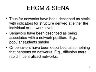
ERGM & SIENA. Thus far networks have been described as static with indicators for structure derived at either the individual or network level. Behaviors have been described as being associated with a network position. E.g., popular students smoke

ERGM & SIENA
E N D
Presentation Transcript
ERGM & SIENA • Thus far networks have been described as static with indicators for structure derived at either the individual or network level. • Behaviors have been described as being associated with a network position. E.g., popular students smoke • Or behaviors have been described as something that happens on networks. E.g., diffusion more rapid in centralized networks.
Co-evolution • Yet, we know that both behaviors and networks evolve and are related. • And, we want an estimation of the likelihood for certain network, behavioral, and/or network-behavioral. • The Exponential Random Graph Model (ERGM) framework provides the framework to address these issues. • ERGM make extensive use of computer simulation and generates random networks are created to make statistical conclusions about the observed/empirical data.
ERGM • ERGM= Exponential Random Graph Models • Random Graph = creating randomly generated networks • Exponential because they are based on an exponential distribution, that is the log of the ratio of probabilities
Key Features • Statistical test is for the probability of a tie between 2 nodes. • What is the likelihood a tie exists given a set of conditions. • To calculate the probability, a large set of random networks need to be generated to make the comparison
ERGM • Test hypotheses about network structure. E.g., Does this network exhibit more reciprocity than would be expected by chance? • Test hypotheses about behavior. E.g., is friend smoking associated with individual smoking?
P1, P*, PNET, ERGM, SIENA • Two competing teams developing software for hypotheses testing • PNET/ERGM consist of Gary Robbins (Australia) and others • SIENA (StocNet) consist of Tom Snijders (Oxford and U. Gronigen, Netherlands) and others
Network Characteristics Density Reciprocity Transitivity 2-stars Other Network Properties A B Antecedents: Sex Age Ethnicity Socio-Economic Status Other Characteristics Individual Behaviors Smoking Sexual Risk Screening Other Behaviors
Crouch, Wasserman & Contractor () • Explains how p* works • Quick review of logistic regression • Provides hypothetical example • Empirical example
Network 1 2 3 4 5 6 - - - - - - 1 0 1 1 0 0 0 2 1 0 1 0 0 0 3 0 1 0 1 0 1 4 0 0 0 0 1 1 5 0 0 0 1 0 0 6 0 0 1 1 0 0 N=6 L=12 Potential Links N(n-1)=6*5=30
Network is a function of: • Overall Density • Mutuality • Transitivity • Cycles • … • In other words, given certain densities, reciprocities, transitivities, etc., we can recreate the empirical network
Links are also function of properties • Since the overall network is a function of density, mutuality, etc. • We can examine any individual tie in the network as a function of these properties Tie is a function of choice, choice w/n attribute, mutuality, mutuality w/n attrib, etc.
And here is the tricky part • To estimate the model we examine how each parameter changes when the links are changed • Step through every dyadic relationship • Calculate how the parameters (density, mutuality, etc.) change • Then regress the links on these change parameters
Statistical Model is: • Tie = Choice Choice_Within Mutuality Mutuality_Within Transitivity • Ties are binary so we use logistic regression
Logit Analysis in STATA(note difference than Crouch et al.) logit tie l l_w m m_w t_t note: l dropped due to collinearity Iteration 0: log likelihood = -20.19035 Iteration 1: log likelihood = -11.068955 Iteration 2: log likelihood = -10.49291 Iteration 3: log likelihood = -10.446967 Iteration 4: log likelihood = -10.44628 Iteration 5: log likelihood = -10.44628 Logistic regression Number of obs = 30 LR chi2(4) = 19.49 Prob > chi2 = 0.0006 Log likelihood = -10.44628 Pseudo R2 = 0.4826 ------------------------------------------------------------------------------ tie | Coef. Std. Err. z P>|z| [95% Conf. Interval] -------------+---------------------------------------------------------------- l_w | 2.740574 2.183488 1.26 0.209 -1.538985 7.020132 m | 3.736891 1.82861 2.04 0.041 .1528821 7.3209 m_w | -1.58782 2.921087 -0.54 0.587 -7.313046 4.137406 t_t | -.408487 .6896983 -0.59 0.554 -1.760271 .9432968 _cons | -2.20826 1.19699 -1.84 0.065 -4.554317 .1377973 ------------------------------------------------------------------------------
There are standard parameter settings Note. See Snijders et al. (2006) and Robins, Pattison, & Wang (in press) for additional information on model parameters.
From Static to Dynamic • So in a single network, we can regress the probability of a tie between 2 actors as a function of several network properties. • What about longitudinally? • Can we model the probability of a tie at time 2 based on these same types of network properties?
Yes, MCMC • To model network dynamics, we employ Markov Chain Monte Carlo (MCMC) • The Markov model states that a particular network configuration is a function of that network at the prior time period. • We can generate a series of micro-steps which are small changes in the network and behavior to mimic how the data evolved from time 1 to time 2.
In SIENA: • One specifies the objective function: The network tendencies (reciprocity, transitivity, etc.). • One specifies the rate function: The frequency of network and/or behavioral changes.
The Simulation • SIENA generates hundreds of possible network and behavioral configurations at each step • This dataset of randomly generated networks is compared to the empirical one and a t-test calculated. • The average of these t-tests over the entire simulation is calculated to determine if there is a tendency in the data to conclude a structural or behavioral effect.
Exposure v. ERGM • The exposure model we regress behavior on the number or percent of ties that engage in the behavior • The dyadic model we regress behavior on whether the dyad engages in the behavior • In ERGM we use the behavior as an attribute and determine whether links are more likely among nodes with the same attribute • It is a homophily test.
Subtle but Important Difference: • The ERGM model allows the researcher to include higher order structural properties such as mutuality, transitivity, etc. • The exposure model allows easier weighting of individual and alter attributes (e.g., is association between behaviors stronger for same sex dyads). • Currently probably need to do both types of analysis
Recent Developments • Special Issue of Social Networks May 2007 Vol. 29 • General introduction • More parameters (2-stars, 2-,3-,4- triangles) • Multiple networks
Empirical NxN Matrix of Ties 100 Randomly Generated NxN Matrices Matched Density Reciprocity Transitivity 2-Stars Density Reciprocity Transitivity 2-Stars Matched Tested Tested
The Actor-Oriented Co-evolution Model: • Provided the opportunity to control for network dependencies not previously controlled. • Provided a means to compare selection and influence.