Approaches for Nanomaterials Modeling
630 likes | 772 Vues
Approaches for Nanomaterials Modeling. Scott Dunham Professor, Electrical Engineering Adjunct Professor, Materials Science & Engineering Adjunct Professor, Physics University of Washington. Introduction. Modeling and simulation provides powerful tool for process/device development.

Approaches for Nanomaterials Modeling
E N D
Presentation Transcript
Approaches for Nanomaterials Modeling Scott Dunham Professor, Electrical Engineering Adjunct Professor, Materials Science & Engineering Adjunct Professor, Physics University of Washington
Introduction • Modeling and simulation provides powerful tool for process/device development. • In semiconductor industry, this is called Technology Computer Aided Design. • Essential to rapid advancement of technology. • Crucible for development of new approaches. • Can we build on that foundation to efficiently develop understanding and tools for Nanotechnology? • Apply modeling at several levels: • First principles (DFT) calculations of physical and electronic structure to guide. • Empirical atomistic simulations: molecular dynamics (MD) • Mesoscale models to span time/spatial scales (e.g., MC) • Continuum simulation of functional systems.
Process Schedule Device Structure Electrical Characteristics Device Simulator Process Simulator VLSI Technology CAD Current semiconductor processes/devices designed via technology computer aided design (TCAD) 1. 30 min, 1000C, O2 2. CVD Nitride, 800C, 20 min 3. Implant 2keV, 21015 As 4. … • Similar tools for design of other nano systems would be extremely powerful.
Ab-initio (DFT) Modeling Approach Expt. Effect Behavior Validation & Predictions Critical Parameters Model DFT Ab-initio Method: Density Functional Theory (DFT) Parameters Verify Mechanism
Modeling Hierarchy * accessible time scale within one day of calculation
Modeling Hierarchy Induced strains, binding/migration energies. Configuration energies and transition rates. Nanoscale Behavior Calibration/testing of empirical potentials Behavior during regrowth, atomistic vs. global stress Configuration energies and transition rates
Multi-electron Systems Hamiltonian (KE + e-/e- + e-/Vext): Hartree-Fock—build wave function from Slater determinants: The good: • Exact exchange The bad: • Correlation neglected • Basis set scales factorially [Nk!/(Nk-N)!(N!)]
DFT: Density Functional Theory Problem: For more than a couple of electrons, direct solution of Schrödinger Equation intractible: (r1,r2,…,rn). Solution: Hohenberg-Kohn Theorem There exists a functional for the ground state energy of the many electron problem in terms of the electron density: E[n(r)]. Caveat: No one knows what it is, but we can make guess … Hamiltonian: Functional: P. Hohenberg and W. Kohn, Phys. Rev. 136, B864 (1964)
Hohenberg-Kohn Theorem Theorem: There is a variational functional for the ground state energy of the many electron problem in which the varied quantity is the electron density. Hamiltonian: N particle density: Universal functional: P. Hohenberg and W. Kohn,Phys. Rev. 136, B864 (1964)
Density Functional Theory Kohn-Sham functional: with Different exchange functionals: Local Density Approx. (LDA) Local Spin Density Approx. (LSD) Generalized Gradient Approx. (GGA) Walter Kohn W. Kohn and L.J. Sham, Phys. Rev. 140, A1133 (1965)
Arrangement of atoms Guess: Electronic Iteration Self-consistent KS equations: Ionic Iteration • Determine ionic forces • Ionic movement Calculation converged Implementation of DFT in VASP VASP features: • Plane wave basis • Ultra-soft Vanderbilt type pseudopotentials • QM molecular dynamics (MD) • VASP parameters: • Exchange functional (LDA, GGA, …) • Supercell size (typically 64 Si atom cell) • Energy cut-off (size of plane waves basis) • k-point sampling (Monkhorst-Pack)
Sample Applications of DFT • Idea:Minimize electronic energy of given atomic structure • Applications: • Atomic Structure (a) • Formation energies (b) • Transitions (c) • Band structure (d) • Charge distributions (e) • … (a) (e) (b) (c) (d)
Sample Applications of DFT • Idea:Minimize energy of given atomic structure • Applications: • Formation energies (a) • Transitions (b) • Band structure (c) • Elastic properties (talk) • … (a) (b) (c)
DFT: Only as good as its results Cohesive energy: J.P. Perdew et al., Phys. Rev. Lett. 77, 3865 (1996) Silicon properties:
Predictions of DFT Atomization energy: J.P. Perdew et al., Phys. Rev. Lett. 77, 3865 (1996) Silicon properties:
Elastic Properties of Silicon Lattice constant: Hydrostatic: Elastic properties: Uniaxial: GGA GGA
Behavior of F Implanted in Si Potential Advantages: • F retards B and P diffusion • F enhances B activation (Huang et al.) Mysterious F behavior: • Exhibits anomalous diffusion • Retards/enhances B, P diffusion Experiment: 30keV F+ implant anneal Data from Jeng et al.
Fluorine Reference Structure Lowest energy structure of single F: • F in bond-centered interstitial site (0.18eV preference over tetrahedral site) • Diffusion barrier of highly mobile
Charge State of F in Si Lowest energy structure of single F: • F+ in bond-centered interstitial site (p-type material) • F- in tetrahedral interstitial site (n-type material) • Diffusion barrier of highly mobile
FnVm Clusters Idea: Fluorine decoration of vacancies immobile clusters FnVm clusters are formed via decoration of dangling Si bonds Ab-initio binding energies: Reference: Fi, V or V2 • Results: • FnVm clusters have large binding • energies
Charge States Analysis FnVm Idea: Fluorine decoration of vacancies immobile clusters For mid gap Fermi level dominant clusters are uncharged Reference:Fi, V and V2
Extended Fluorine Continuum Model Formation: Dissociation: Diffusion of Mobile F, I, V Defect Model & Boundary Conditions: • Extended defect model including In, Vn, and {311} defects • Thin oxide layer on surface (20 Å) (segregation & diffusion of Fi)
Fluorine Redistribution Simulation: Experiment: Fluorine diffusion mechanism: • Fast diffusing Fi get trapped in V • Release Fi via I • F decoration of V leads to F dissolving from deeper regions (I excess) and accumulation near surface (V excess) V rich I rich
F Effect on B and P Possible effects on dopant redistribution: • Direct interaction via B-F and P-F binding • Indirect interaction via point-defect modifications Ab-initio calculation: No significant binding energies indirect mechanism F alters local point-defect concentration Prediction: • F model should explain effect of F on B and P comprehensively
Simplified Fluorine Model F dose time evolution: Interaction Mechanism: 30min anneal at 650°C After 20s, F3V and F6V2 Dissolution reaction: Key parameter: a/c interface F profile depth
Fluorine Diffusion • Experiment: • 20keV 3x1015cm-2 F • implant • 1050°C spike anneal • No other dopants
F Effect on Phosphorus Source/Drain Pocket
F Effect on Boron Source/Drain Pocket
Summary: Fluorine Model Tasks: • Identified F diffusion mechanism • Developed simplified F model to understand F effect on P and B • Modeled range of experimental data (Texas Instruments) Simplified F model: • Comprehensive treatment of amorphous and sub-amorphous conditions • a/c depth and F profile are key parameters to understand F effect Results: • F diffusion can be understood via FnVm clusters • F affects P and B diffusion indirectly via modification of local point-defect concentrations
Peptide-Surface Interactions • Apply hierarchical approaches to understanding/modeling peptide binding to inorganic surfaces • First step is to explore via DFT calculations • Interesting problem is specific binding to different noble metals (Au, Ag, Pt). • List of strong/weak binding trimers and quadramers (Oren) • Picked Arginine (R) as first to explore
Peptide-Surface Interactions • Structure from MD (Oren) • Distinctive 3N structures • Explore via DFT
Peptide-Surface Interactions • Truncated arginine with O acceptor. • 111 Au surface (upper layers free)…no H2O • VASP-GGA structure minimization (limited)
Peptide-Metal Interactions • Explore basis for peptide binding to metals. • Charge distribution with and without arginine. • Fractional charge transferred to O (~0.2e-) • Small induced charge on metal (exploring further…)
Peptide-Metal Interactions • 3D Charge distribution for peptide/surface system
MD Simulation Initial Setup Stillinger-Weber or Tersoff Potential 5 TC layer 1 static layer 4 x 4 x 13 cells Ion Implantation (1 keV)
Recrystallization 1200K for 0.5 ns
MD Results: Regrowth of Si:As • As Diffusion in a-Si • Enhanced relative to c-Si. • As Bonding • As coordination close to 3 in amorphous • Changes to 4 in crystalline Si. • V Incorporation • No vacancies for low As concentrations • Grown-in AsnV clusters at high CAs.
Fi, E DFT Error Optimizer Configs. Fi, E MD Parameters Molecular Dynamics • MD widely and effectively used for organic molecules and inorganic materials. • A key challenge is accurate (transferable) interatomic potentials • A solution is use of DFT for calibration.
Empirical Potential Optimization • Data set for training includes: • Lattice constant, structure • Elastic properties (stiffness tensor) • Point defect formation energies • Configurations from high T ab-initio MD • Match to both energies and forces. • Start with pure Si and then add impurities one-by-one
Time Scale Issue • Systems evolves slowly because there are local metastable states with long lifetime (high barriers relative to kT). • Also need to follow atomic vibrations (fs) • Can speed up by only considering only transitions.
Temperature Accelerated Dynamics • TAD (Sorenson and Voter) speeds up MD by running system at higher T to find transitions. • Multiple high T runs to identify possible transitions. • Actual transition chosen based on lower T under study. • Need enough to ensure finding low barrier process which dominates at lower T. • Acceleration factors of 107 or more possible (depends on ΔE and T).
Dimer Method • Create “dimer” of system in configurational space near energy minimum. • Minimize energy of dimer keeping center fixed. • Finds lowest curvature direction (Voter 1997). • Invert force component along dimer to define ‘effective force’. • Minimize effective force. Mirror Plane Henkelman and Jónsson, JCP 111, 7010 (1999)
Find saddle points using dimer method. Calculate transition rates. Use random number to choose transitions. Advance system. Increment time. Repeat 1 to 5, until t = tmax. Adaptive Kinetic Monte Carlo Henkelman & Jonsson., JCP.115, 9657 (2001).
Need for Mesoscale Models Some problems are too complex to connect DFT directly to continuum. • High C, alloys, discrete effects, peptide binding MD suffers from time scale dilemma: need to follow atomic vibrations (t~10-100fs) • Need a scalable atomistic approach. Apply Transition State Theory. • Only follow major transitions
Kinetic Lattice Monte Carlo (KLMC) • With crystal lattice, there is countable set of transitions • Energies/hop rates from DFT • Much faster than MD because: • Only consider defects • Only consider transitions • Develop discrete model for energy vs. configuration • Base hop rates vary with E
KLMC Simulations Set up crystal lattice structure (10-50nm)3 Defects (dopant and point defects) initialized - based on equilibrium concentration - or imported from implant simulation - or user-defined
Kinetic Lattice Monte Carlo Simulations KLMC Simulations Simulations include B, As, I, V, Bi, Asi and interactions between them. Hop/exchange rate determined by change of system energy due to the event. Energy depends on configuration with numbers from ab-initio calculation (interactions up to 9NN).
Kinetic Lattice Monte Carlo Simulations KLMC Simulations Calculate rates of all possible processes. At each step, Choose a process at random, weighted by relative rates. Increment time by the inverse sum of the rates. Perform the chosen process and recalculate rates if necessary. Repeat until conditions satisfied.
High Concentration As Diffusion • DFT shows long-range As/V binding • Possible configurations too numerous for simple analysis. • Can use Kinetic Lattice Monte Carlo (KLMC) simulation.
Acceleration of KLMC Simulations Problem: Once a cluster is formed, the system can spend a long time just making transitions within a small group of states.