Download
1 / 50
500 likes | 638 Vues
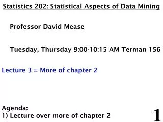
Statistics 202: Statistical Aspects of Data Mining Professor David Mease Tuesday, Thursday 9:00-10:15 AM Terman 156 Lecture 3 = More of chapter 2 Agenda: 1) Lecture over more of chapter 2. Homework Assignment: Chapters 1 and 2 homework is due Tuesday 7/10

E N D
Statistics 202: Statistical Aspects of Data Mining Professor David Mease Tuesday,Thursday 9:00-10:15AM Terman 156 Lecture 3 = More of chapter 2 Agenda: 1) Lecture over more of chapter 2
Homework Assignment: Chapters 1 and 2 homework is due Tuesday 7/10 Either email to me (dmease@stanford.edu), bring it to class, or put it under my office door. SCPD students may use email or fax or mail. The assignment is posted at http://www.stats202.com/homework.html
Introduction to Data Mining by Tan, Steinbach, Kumar Chapter 2: Data
What is Data? • An attribute is a property or characteristic of an object • Examples: eye color of a person, temperature, etc. • Attribute is also known as variable, field, characteristic, or feature • A collection of attributes describe an object • Object is also known as record, point, case, sample, entity, instance, or observation Attributes Objects
Types of Attributes: • Qualitative vs. Quantitative (P. 26) • Qualitative (or Categorical) attributes represent distinct categories rather than numbers. Mathematical operations such as addition and subtraction do not make sense. Examples: eye color, letter grade, IP address, zip code • Quantitative (or Numeric) attributes are numbers and can be treated as such. Examples: weight, failures per hour, number of TVs, temperature
Types of Attributes (P. 25): • All Qualitative (or Categorical) attributes are either Nominalor Ordinal. • Nominal = categories with no order • Ordinal = categories with a meaningful order • AllQuantitative (or Numeric) attributes are either Interval or Ratio. • Interval = no “true” zero, division makes no sense • Ratio = true zero exists, division makes sense
Types of Attributes: • Some examples: • Nominal • Examples: ID numbers, eye color, zip codes • Ordinal • Examples: rankings (e.g., taste of potato chips on a scale from 1-10), grades, height in {tall, medium, short} • Interval • Examples: calendar dates, temperatures in Celsius or Fahrenheit, GRE score • Ratio • Examples: temperature in Kelvin, length, time, counts
Properties of Attribute Values • The type of an attribute depends on which of the following properties it possesses: • Distinctness: = • Order: < > • Addition: + - • Multiplication: * / • Nominal attribute: distinctness • Ordinal attribute: distinctness & order • Interval attribute: distinctness, order & addition • Ratio attribute: all 4 properties
Discrete vs. Continuous (P. 28) • Discrete Attribute • Has only a finite or countably infinite set of values • Examples: zip codes, counts, or the set of words in a collection of documents • Often represented as integer variables • Note: binary attributes are a special case of discrete attributes which have only 2 values • Continuous Attribute • Has real numbers as attribute values • Can compute as accurately as instruments allow • Examples: temperature, height, or weight • Practically, real values can only be measured and represented using a finite number of digits • Continuous attributes are typically represented as floating-point variables
Discrete vs. Continuous (P. 28) • Qualitative (categorical) attributes are always discrete • Quantitative (numeric) attributes can be either discrete or continuous
In class exercise #3: Classify the following attributes as binary, discrete, or continuous. Also classify them as qualitative (nominal or ordinal) or quantitative (interval or ratio). Some cases may have more than one interpretation, so briefly indicate your reasoning if you think there may be some ambiguity. a) Number of telephones in your house b) Size of French Fries (Medium or Large or X-Large) c) Ownership of a cell phone d) Number of local phone calls you made in a month e) Length of longest phone call f) Length of your foot g) Price of your textbook h) Zip code i) Temperature in degrees Fahrenheit j) Temperature in degrees Celsius k) Temperature in Kelvins
Types of Data in R • R often distinguishes between qualitative (categorical) attributes and quantitative (numeric) • In R, qualitative (categorical) =“factor” quantitative (numeric) =“numeric”
Types of Data in R • For example, the IP address in the first column of www.stats202.com/stats202log.txt is a factor • > data<-read.csv("stats202log.txt", • sep=" ",header=F) • > data[,1] • [1] 69.224.117.122 69.224.117.122 69.224.117.122 128.12.159.164 128.12.159.164 128.12.159.164 128.12.159.164 128.12.159.164 128.12.159.164 128.12.159.164 • … • … • [1901] 65.57.245.11 65.57.245.11 65.57.245.11 65.57.245.11 65.57.245.11 65.57.245.11 65.57.245.11 65.57.245.11 65.57.245.11 65.57.245.11 • [1911] 65.57.245.11 67.164.82.184 67.164.82.184 67.164.82.184 171.66.214.36 171.66.214.36 171.66.214.36 65.57.245.11 65.57.245.11 65.57.245.11 • [1921] 65.57.245.11 65.57.245.11 • 73 Levels: 128.12.159.131 128.12.159.164 132.79.14.16 171.64.102.169 171.64.102.98 171.66.214.36 196.209.251.3 202.160.180.150 202.160.180.57 ... 89.100.163.185 • > is.factor(data[,1]) • [1] TRUE > data[,1]+10 [1] NA NA NA NA NA NA NA NA… Warning message: + not meaningful for factors …
Types of Data in R • However, the 8th column looks like it should be numeric. Why is it not? How do we fix this? • > data[,8] • [1] 2867 4583 2295 2867 4583 2295 1379 2294 4432 7134 2296 2297 3219968 1379 2294 4432 7134 2293 2297 2294 … • [1901] 2294 4432 7134 2294 4432 7134 2294 2867 4583 2295 2294 4432 7134 2294 4432 7134 2294 2294 2294 2294 • [1921] 2294 2294 • Levels: - 1135151 122880 1379 1510 2290 2293 2294 2295 2296 2297 2309 238 241 246 248 250 2725487 280535 2867 3072 3219968 4432 4583 626 7134 7482 • > is.factor(data[,8]) • [1] TRUE • > is.numeric(data[,8]) • [1] FALSE
Types of Data in R • A: We should have told R that “-” means missing when we read it in. • > data<-read.csv("stats202log.txt", • sep=" ",header=F, na.strings = "-") • > is.factor(data[,8]) • [1] FALSE • > is.numeric(data[,8]) • [1] TRUE
Types of Data in R • Q: How would we create an attribute giving the following zip codes 94550, 00123, 43614 for three observations in R?
Types of Data in R • Q: How would we create an attribute giving the following zip codes 94550, 00123, 43614 for three observations in R? • A: Use quotes: • > zip_codes<- as.factor(c("94550","00123","43614"))
Types of Data in Excel • Excel is not quite as picky and allows you to mix types more • Also, you can change between a lot of different predefined formats in Excel by right clicking a column and then selecting “Format Cells” and looking under the “Number” tab
Types of Data in Excel • Q: How would we create an attribute giving the following zip codes 94550, 00123, 43614 for three observations in Excel?
Types of Data in Excel • Q: How would we create an attribute giving the following zip codes 94550, 00123, 43614 for three observations in Excel? • A: Right click on the column then choose “Format Cells” then under the “Number” tab select “Text”
Working with Data in R Creating Data: > aa<-c(1,10,12) > aa [1] 1 10 12 Some simple operations: > aa+10 [1] 11 20 22 > length(aa) [1] 3
Working with Data in R Creating More Data: > bb<-c(2,6,79) > my_data_set<-data.frame(attributeA=aa,attributeB=bb) > my_data_set attributeA attributeB 1 1 2 2 10 6 3 12 79
Working with Data in R Indexing Data: > my_data_set[,1] [1] 1 10 12 > my_data_set[1,] attributeA attributeB 1 1 2 > my_data_set[3,2] [1] 79 > my_data_set[1:2,] attributeA attributeB 1 1 2 2 10 6
Working with Data in R Indexing Data: > my_data_set[c(1,3),] attributeA attributeB 1 1 2 3 12 79 Arithmetic: > aa/bb [1] 0.5000000 1.6666667 0.1518987
Working with Data in R Summary Statistics: > mean(my_data_set[,1]) [1] 7.666667 > median(my_data_set[,1]) [1] 10 > sqrt(var(my_data_set[,1])) [1] 5.859465
Working with Data in R Writing Data: > setwd("C:/Documents and Settings/Administrator/Desktop") > write.csv(my_data_set,"my_data_set_file.csv") Help!: > ?write.csv
Working with Data in Excel Reading in Data:
Working with Data in Excel Deleting a Column: (right click)
Working with Data in Excel Arithmetic:
Working with Data in Excel Summary Statistics: Use “Insert” then “Function” then “All” or “Statistical” to find an alphabetical list of functions
Working with Data in Excel Summary Statistics: (Average)
Working with Data in Excel Summary Statistics: (Median)
Working with Data in Excel Summary Statistics: (Standard Deviation)
Sampling (P.47) • Sampling involves using only a random subset of the data for analysis • Statisticians are interested in sampling because they often can not get all the data from a population of interest • Data miners are interested in sampling because sometimes using all the data they have is too slow and unnecessary
Sampling (P.47) • The key principle for effective sampling is the following: • using a sample will work almost as well as using the entire data sets, if the sample is representative • a sample is representative if it has approximately the same property (of interest) as the original set of data
Sampling (P.47) • The simple random sample is the most common and basic type of sample • In a simple random sample every item has the same probability of inclusion and every sample of the fixed size has the same probability of selection • It is the standard “names out of a hat” • It can be with replacement (=items can be chosen more than once) or without replacement (=items can be chosen only once) • More complex schemes exist (examples: stratified sampling, cluster sampling, Latin hypercube sampling)
Sampling in Excel: • The function rand() is useful. • But watch out, this is one of the worst random number generators out there. • To draw a sample in Excel without replacement, use rand() to make a new column of random numbers between 0 and 1. • Then, sort on this column and take the first n, where n is the desired sample size. • Sorting is done in Excel by selecting “Sort” from the “Data” menu
Sampling in R: • The function sample() is useful.
In class exercise #4: Explain how to use R to draw a sample of 10 observations with replacement from the first quantitative attribute in the data set www.stats202.com/stats202log.txt.
In class exercise #4: Explain how to use R to draw a sample of 10 observations with replacement from the first quantitative attribute in the data set www.stats202.com/stats202log.txt. Answer: > sam<-sample(seq(1,1922),10,replace=T) > my_sample<-data$V7[sam]
In class exercise #5: If you do the sampling in the previous exercise repeatedly, roughly how far is the mean of the sample from the mean of the whole column on average?
In class exercise #5: If you do the sampling in the previous exercise repeatedly, roughly how far is the mean of the sample from the mean of the whole column on average? Answer: about 26 > real_mean<-mean(data$V7) > store_diff<-rep(0,10000) > > for (k in 1:10000){ + sam<-sample(seq(1,1922),10,replace=T) + my_sample<-data$V7[sam] + store_diff[k]<-abs(mean(my_sample)-real_mean) + } > mean(store_diff) [1] 25.75126
In class exercise #6: If you change the sample size from 10 to 100, how does your answer to the previous question change?
In class exercise #6: If you change the sample size from 10 to 100, how does your answer to the previous question change? Answer: It becomes about 8.1 > real_mean<-mean(data$V7) > store_diff<-rep(0,10000) > > for (k in 1:10000){ + sam<-sample(seq(1,1922),100,replace=T) + my_sample<-data$V7[sam] + store_diff[k]<-abs(mean(my_sample)-real_mean) + } > mean(store_diff) [1] 8.126843
The square root sampling relationship: • When you take samples, the differences between the sample values and the value using the entire data set scale as the square root of the sample size for many statistics such as the mean. • For example, in the previous exercises we decreased our sampling error by a factor of the square root of 10 (=3.2) by increasing the sample size from 10 to 100 since 100/10=10. This can be observed by noting 26/8.1=3.2. • Note: It is only the sizes of the samples that matter, and not the size of the whole data set (the population) since this relationship assumes an infinitely large population.
Sampling (P.47) • Sampling can be tricky or ineffective when the data has a more complex structure than simply independent observations. • For example, here is a “sample” of words from a song. Most of the information is lost. oops I did it again I played with your heart got lost in the game oh baby baby oops! ...you think I’m in love that I’m sent from above I’m not that innocent
Sampling (P.47) • Sampling can be tricky or ineffective when the data has a more complex structure than simply independent observations. • For example, here is a “sample” of words from a song. Most of the information is lost. oops I did it again I played with your heart got lost in the game oh baby baby oops! ...you think I’m in love that I’m sent from above I’m not that innocent