Download
1 / 25
250 likes | 351 Vues
This presentation delves into the performance metrics of two types of backpressure routing protocols and the errors encountered during their operation. It defines key concepts such as queue backlogs, channel rates, and arrival/service rates in a network of mobile nodes. The analysis focuses on error types affecting control information dissemination and their impact on network efficiency. Through simulation, the paper evaluates the effectiveness of two distinct control information distribution protocols: one using a fixed-time approach and the other adopting a time-stamped method. The findings enhance understanding of network dynamics and error management in distributed systems.

E N D
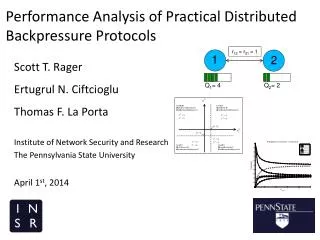
Performance Analysis of Practical Distributed Backpressure Protocols r12 = r21 = 1 Scott T. Rager ErtugrulN. Ciftcioglu Thomas F. La Porta Institute of Network Security and Research The Pennsylvania State University April 1st, 2014 Q1= 4 Q2= 2 2 1
This talk will focus on analyzing two kinds of errors in Backpressure Routing and their impact Overview on Backpressure Routing Two Control Information Dissemination Protocols Characterizing Errors VS. Probability and Impact of Errors
First, we need some definitions and assumptions Network Setup: ... We assume a network on N mobile nodes that operates in discrete time slots Q1=1 Qi(t) = Queue backlog of node i at time t (can be packets or bits – doesn’t matter) r12=2 rij(t) = available channel rate from node i to node j at time t μij(t) = scheduled channel rate from node i to node j at time t μ12=0 λi λi(t) = arrival rate from application to node i at time t ai(t) = arrivals from other nodes to node i at time t bi(t) = service rate of node i at time t bi Assumptions: We assume λmax < bmax and λavg< bavg 1 2 N
Backpressure is a max-weight sum of queue differences and channel rates Choose valid set of transmission rates that: Largest max-weight = optimum schedule Example: (Q1-Q2)*μ12 = (4 – 2)*1 = 2 (Q1-Q2)*μ12 = (4 – 2)*1 = 2 (μ12 = 0) r12 = r21 = 1 (Q2-Q1)*μ21 = (2 – 4)*1 = -2 Otherwise, set of rates would cause a collision and would not be valid Q1= 4 Q2= 2 Queue Update: *sums from τ= t to t+τ-1 Qn(t+1) = max{Qn(t) – bn(t), 0} + an(t) + λn(t) Queue Drift Bound: 2 Qn(t+T) = max{Qn(t) – Σ(bn(t)), 0} + Σ(an(t) ) + Σ(λn(t)) * 1
Backpressure Routing provides a number of benefits of traditional network approaches Operates on instantaneous network state Throughput Optimal Can modify to consider utility or power consumption, too: QoI No need for a priori knowledge of network dynamics
...but it’s not all good Requires Global Knowledge of network state (queue backlogs and channel rates) μ13=5 Need to distribute this network state, or control information to make decisions distributedly, which: μ12=5 Q2=5 μ23=4 μ14=1 Q3=2 Q3=4 μ34=3 Q3 Q2 Q4 1. Leads to overhead 1 μ14=1 2. In practical applications, errors exist, which lead to impact on performance μ13=5 4 μ12=5 μ34=3 3 μ23=4 2
The first protocol to distribute control information is a fixed-time, best effort approach If all backlog information is exchanged, then each node can find the optimal schedule in a distributed fashion. If the network runs out of time before it completely disseminates the information, then some nodes’ backlogs values have errors that cause inconsistent views of the network. Each node repeatedly broadcasts known queue backlogs from this time slot using CSMA to attempt to avoid collisions. Uses fixed amount of time for exchanging control information Example: 6 3 3 5 6 TCtrl • TData 5 5 1 4 3 2 5 TSlot
The second protocol to distribute control information sends one packet of time-stamped values each time slot Here, all nodes keep a window of control information for previous T slots and exchange queue values with time-stamps. The farthest distance between nodes is N-1 hops, so setting T=N-1 ensures that all nodes will have consistent views of the network. Note that these views will be outdated, and, therefore, contain errors. 2 3 4 1
We simulated each of the protocols in an attempt to characterize the errors that each generate Approximated as Normal RV Approximated as Uniform RV Best Effort Protocol (Inconsistent Information) Delayed Info Protocol (Consistent Information)
Let’s use a motivating example to compare the two control information dissemination protocols Take the simplest case of two nodes with equivalent channel rates. Q1=5 Q2=4 μ12=μ21=1 Q2= 5 Q2= 4 When Q1 > Q2, then Node 1 transmits, Node 2 is silent, and full throughput is achieved. What happens if we introduce errors? 2 1
What happens when the network uses the best effort protocol and errors are inconsistent: Let ei(j) = the error in Queue i at Node j Case A: Let e1(2) = 1 e2(1) = 0 Q1= 5 Q1 = 6 Q2=4 μ12=μ21=1 Then: Node 1 transmits Node 2 is silent Full throughput is achieved. Q2= 5 Q2= 4 2 1
What happens when the network uses the best effort protocol and errors are inconsistent: Let ei(j) = the error in Queue i at Node j Case B: Let e1(2) = -2 e2(1) = 2 Q1 = 3 Q1= 5 Q2=6 Q2=4 μ12=μ21=1 Then: Node 1 is silent Node 2 transmits The schedule is not optimal, but the channel is fully utilized with no collisions. Q2= 5 Q2= 4 2 1
What happens when the network uses the best effort protocol and errors are inconsistent: Let ei(j) = the error in Queue i at Node j Case C: Collision Let e1(2) = -2 e2(1) = 0 Q1 = 3 Q1= 5 Q2=4 Q2=4 μ12=μ21=1 Then: Node 1 transmits Node 2 transmits Both nodes believe they should transmit, resulting in a collision and no effective use of the channel. Q2= 5 Q2= 4 2 1
What happens when the network uses the best effort protocol and errors are inconsistent: Let ei(j) = the error in Queue i at Node j Case D: Let e1(2) = 0 e2(1) = 2 Q1= 5 Q2=6 Q2=4 μ12=μ21=1 Then: Node 1 is silent Node 2 is silent Both nodes defer believing the other should transmit resulting in dead air and no utilization of the channel. Q2= 5 Q2= 4 2 1
Summary of outcomes for Inconsistent Information with varying errors Note that two outcomes result in zero effective use of the channel.
What happens when the network uses the best effort protocol and errors are inconsistent: Let ei = the error in Queue i at both Nodes Case A: Let e1 = 2 e2 = 0 Q1 = 7 Q1= 5 Q2=4 μ12=μ21=1 Then: Node 1 transmits Node 2 is silent Full throughput is achieved. Q1 = 7 Q1= 5 Q2= 4 2 1
What happens when the network uses the best effort protocol and errors are inconsistent: Let ei = the error in Queue i at both Nodes Case B: Let e1 = 0 e2 = 2 Q1= 5 Q2=4 Q2=6 μ12=μ21=1 Then: Node 1 is silent Node 2 transmits The schedule is not optimal, but the channel is fully utilized with no collisions. Q1= 5 Q2= 4 Q2= 6 2 1
Summary of outcomes for Inconsistent Information with varying errors Here all outcomes result in fully using the channel.
Using the characterization from the empirical observations, we can develop an expression of the probability of each outcome • Inconsistent Information: • Using Normal RV with standard deviation, EStdDev • CDF of error becomes: As the error bound grows: Probability of each case
Summary of outcomes for Inconsistent Information with varying errors Note that two outcomes result in zero effective use of the channel.
Using the characterization from the empirical observations, we can develop an expression of the probability of each outcome • Consistent Information: • Using Uniform RV with standard deviation, EMax • CDF of error becomes: As the error bound grows: Probability of each case *Note: No lost bandwidth
Summary of outcomes for Inconsistent Information with varying errors Here all outcomes result in fully using the channel.
Takeaway 1: “Delayed Info” protocol achieves more throughput Using the Delayed Information to schedule results in higher network capacity. Why? No lost bandwidth from collisions or dead air!
Takeaway 2: Effect of errors dissipates with magnitude for “Inconsistent Info” protocol Small magnitude errors have a distinct impact on performance that diminishes as the error bound increases. Why? No change in outcome once threshold is crossed.
Thank you! Questions?