Download
1 / 31
310 likes | 524 Vues
Trends in Numerical Relativistic Astrophysics. David Meier Jet Propulsion Laboratory Caltech. Introductory Remarks. Purpose of this lecture To discuss some of the numerical astrophysical research our group is doing now and in the near future

E N D
Trends in Numerical Relativistic Astrophysics David Meier Jet Propulsion Laboratory Caltech
Introductory Remarks • Purpose of this lecture • To discuss some of the numerical astrophysical research our group is doing now and in the near future • To indicate where the field might go in the next 10 years or so • To stimulate thinking, especially in the younger members of the audience, on what types of problems and techniques may be addressable in the next 1/3 of a century • Outline • New astrophysics, same physics • New physics, new astrophysics • New numerical techniques on present-day computers • New numerical techniques on future machines • NOTE: few equations will be presented; refer to IPAM tutorial on relativistic astrophysics (Meier 2005a)
I. New Astrophysics, Same Physics • Numerical simulation of magnetized cosmic jets • Non-relativistic flow • Relativistic flow • General Relativistic MHD of accretion disks with cooling • Optically thin cooling: magnetospheres & jet production • Optically thick cooling: “standard” thin, cool disks • Evolving GRMHD and neutron star mergers: effects of magnetic fields
Quasar 1928+738 3C 273 M 87 SUPERMASSIVE BLACK HOLES STELLAR-MASS BLACK HOLES FORMING STARS Virgo A (M87) HH 30 GRS 1915+105 Hummel et al. (1992) © MPIfR © ISAS, CfA PN M2-9 SS 433 Cosmic Jets • Occur in many types of objects DYING & DEADSTARS CRAB PULSAR • Often show “wiggles”
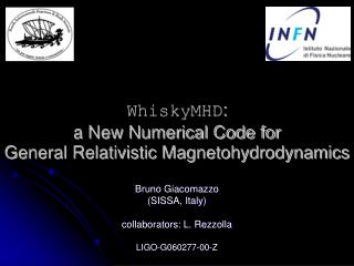
Non-Relativistic MHD Simulations of Cosmic Jets in Decreasing Density Galactic Atmospheres (Nakamura & Meier 2004) • Jet is morestable if density gradient is very steep ( z -3) and jet is mildly PFD (60%) • Jet is moreunstable to m = 1 helical kink if density gradient is shallow ( z -2) and jet is highly Poynting-flux dominated (90%) (helical kink or m=1 current-driven or “screw” instability)
Non-Relativistic MHD Simulations of Cosmic Jets in Decreasing Density Galactic Atmospheres (cont.) • Cause of the instability: “force-free” magnetic field is unstable, but it can be stabilized if the plasma rotates (adds centrifugal force to “radial force balance”) High magnetic field twist + slow rotation Unstable to helical kink High magnetic field twist + rapid rotation More stable to helical kink
Relativistic MHD Simulations of Cosmic Jets in Decreasing Density Galactic Atmospheres • When flow is relativistic, new terms arise in the radial force equation, even without any plasma inertia (force-free!): • When the magnetic field rotation rate v c • Conclusion: Centrifugal force of the magnetic field inertia (B) can balance pinch/hoop stress • Question: Are relativistic magnetized jets self-stabilizing, even without appreciable plasma? We will be investigating this shortly.
GRMHD Simulations of the MRI in Accretion Disks WITH Optically Thin Radiative Cooling • Present-day magneto-rotational instability disk simulations start with a thick torus with a weak magnetic poloidal field and differential (Keplerian) rotation (see IPAM #1 talks by Hawley, Gammie, Stone) • Biggest deficiency of these simulations is the use of an adiabatic energy equation: NO RADIATIVE COOLING • Accreting material remains very hot (1011–13 K), but e– radiate copiously above 1010 K • IF ions couple well to e–, the entire plasma will cool to ~1010–11 K or less • Predicted new structure will have a strong magnetosphere and jet, as seen in real objects A turbulent dynamo develops in a few rotation times (the MRI) McKinney & Gammie (2004) • Question: Does optically thin cooling produce a strong • magnetosphere and jet as predicted by Meier (2005b)? • Need to simulate MRI with GRMHD and cooling.
GRMHD Simulations of the MRI in Accretion Disks WITH Optically Thick Radiative Cooling • The first accretion disks to be modeled analytically (Shakura & Sunyaev 1973) will be the last (and most difficult) ones to simulate numerically: geometrically thin, optically thick • Main scientific and computational issues: • Difficult radiative transfer: • Diffusion in disk interior • Free streaming outside of disk • Must handle photosphere carefully • Coupling between radiation and plasma may be important in luminous disks • Adaptive mesh refinement will be required to properly grid the disk Geometrically Thin Torus Geometrically Thick Torus • Question: Do simulated thin disks behave in the manner predicted by analytic • theory? … as observed in real systems?
EGRMHD Simulations of NS – NS Mergers WITH Magnetic Fields • Virtually ALL observed neutron stars have magnetic fields (109 – 1015 G) • Yet, NO present numerical relativity simulation of NS – NS mergers includes magnetic fields in the dynamics • Examples: Rasio & Shapiro (1999), Shibata et al. (2003), Baumgarte et al. (2004): • Neutron stars merge, but do not form a black hole • Instead, a differentially-rotating, super-NS forms • How will the MRI change things (Balbus & Hawley 1998)? • MRI will create a strong “viscosity”, as in B.H. accretion disks • Fastest growing MRI wavelength and growth rate (B = Bi emaxt) • max VAKepmax = 0.75 Kep • Every rotation, magnetic field will increase by emaxKep = 111 • Even the WEAKEST fields (109 G) will grow to dyn. important strengths (1016 G)in only 3-4 rotation times of the VORTEX • A differentially rotating, super-neutron-star likely will never form. • It will collapse to a black hole in a few dynamical times. • STRONG magnetic fields will likely lead to jets and -ray bursts • Ignoring magnetic fields in relativistic astrophysical simulations is like simulating tar using alcohol. The understanding of B.H. formation critically depends in magnetic processes.
II. New Physics, New Astrophysics • General relativistic charge dynamics • Current sheets in pulsars • Reconnection
General Relativistic Charge Dynamics • GRCD equations (Meier 2004) were introduced in the IPAM tutorial on relativistic astrophysics, derived from the relativistic multi-fluid equations • Fluid equationsT mU = 0 T {TFL + TEM}T = 0 TFL [m+(e+p)/c2]UU + [UH + HU]/c2 + p g] TEM [ F F – ¼ (F : F) I] / (4 ) • Charge equationsT (qU +j) = 0 T CT = p2 { [(1 hq)U + hJ] F/c J } / (4 ) (gen. Ohm’s law) C = [q+(eq+pq)/c2]UU + Uj + jU + pqg (charge/beamed current tensor) • GRCD will be important only on small scales (x < ~ 102–3 D), where 4 |T CT|/ p2 ~ E • For global simulations,x is 105–7times larger, so the standard Ohm’s law will suffice • GRCD will be important primarily in simulations of small-scale phenomena or those with AMR.
PULSAR Current Sheets and Reconnection Phenomena Pulsar Current Sheets • Present simulations (Spitkovsky 2005) have finally solved the pulsar magnetosphere problem; however, they do not resolve the current sheet (where B changes sign) • The current sheet is believed to be a key to understanding the evolution and stability of the pulsar magnetosphere • The GRCD equations have all the physics necessary to simulate the structure and • evolution of the current sheet • But, adaptive Mesh Refinement (AMR), of course, will be needed to resolve the current sheet • One problem: Plasma phenomena occur on very short time scales • Solution: solve the generalized Ohm’s law (T CT = …) as an implicit structure problem, • setting /t = 0 in the Ohm’s law equations. • With this technique, the current sheet will evolve on the pulsar time scale, not on the plasma • time scale • Supersonic Reconnection • When the plasma shear flow is supersonic, |U| > coll (particle collision frequency) and the new Ohm’s Law terms will exceed the regular resistive term: 4 |T CT|/ p2 > J • This is another source of “anomalous” resistivity (scattering off shear flow layers) • This, and other types of anomalous resistivity, may be important in reconnection
III. New Numerical Techniques for EGRD (Numerical Relativity) On Present-day Machines • Constrained Transport and Discrete Exterior Calculus • Simple CT for MHD and full E & M • CT for EGRD (numerical relativity) • Relation to DEC and lattice gauge simulations
Constrained Transport for MHD (Evans & Hawley 1988) • Magnetohydrodynamics (and full electrodynamics) is analogous to numerical relativity in that it has an evolution equation for the field and a constraint that must be satisfied: B = cE B = 0 • Modern MHD codes work by satisfying B = O(r)10-14on the initial hypersurface and then using a differencing scheme that ensures (B) / t = B = c E = O(r) How is this accomplished numerically? Answer: by properly staggering the grid B B 10-14
t0 t½ t1 Bz Bz Bz Bx Bx Bx By By By Az Ez z Ay Ey Ax Ex y x Constrained Transport for MHD (continued) • The grid is staggered in space and time • At t = t0, B = A and B = Bx+Bx + By+By + Bz+Bz = (Az4-Az2) – (Ay4-Ay2) – (Az3-Az1) + (Ay3-Ay1) + (Ax4-Ax2) – (Az4-Az3) – (Ax3-Ax1) + Az2-Az1) + (Ay4-Ay3) – (Ax4-Ax3) – (Ay2-Ay1) + (Ax2-Ax1) = A= O(r) • Then at t = t½, similarly, E= O(r) , so B = O(r) • So, at t = t1, B1 = B0 + t (B½) = O(r) • Proper staggering of the grid creates vector fields in which the divergence of a curl vanishes to machine accuracy, propagating the constraint (vector/Bianchi identity satisfied)
t0 t½ t1 t-½ Bz Bz Bz q, q, q q q Bx Bx Bx By By By Ez , Az , Jz Ez Ez Ez , Jz Ey , Ay , Jy q, Ey , Jy Ey Ey q q Ex Ex Ex , Ax , Jx Ex , Jx CT for Electrodynamics (Yee 1966; Meier 2003) • Problem is more complicated in full electrodynamics: Both of Maxwell’s equations and both of the constraints must be satisfied: B = cE B = 0 E = cB – 4J E = 4c creating the need for three interlaced updates (one each for B, E, and q): 2 = 4q, E =B = AInitialize E = cB – 4JB = cE Evolve q = – J E = 4qB = 0E = 4qB = 0 Implicit E = – 4 JB = 0 E = 4q E = 4q q
t0 t½ t1 t-½ F12 F12 J0, A0 J0, A0 J0 F23 F13 F13 F23 F03 F03 J3 J3, A3 F02 J2, A2 F02 J0, A0 J0 J0 F01 F01 J1, A1 J1 CT for Electrodynamics (continued) • In covariant form, full electrodynamics appears much simpler: F = dAInitialize P (F) = 4 PJP (*F) = 0Evolve J = 0 n (F) = 4n Jn (*F) = 0 (F) = 0 Implicit 4-dimensionalBianchi identities • Staggering the grid implicitly satisfies the Bianchi (and other simpler vector)identities to machine accuracy, and this implicitly propagates the constraints A staggered grid has “deep geometric significance” J0 J2
Staggered Grids in 4-D • The electrodynamics CT problem suggests a natural, simple, and elegant method for staggering finite difference grids in 4-D: Scalars: (hypercube corners) Vectors: (hypercube edges) 2-Tensors: (hypercube faces & corners) tn+½ tn+1 tn J0 J3 J3 J2 J2 1 J0 J0 J1 J1 0 F12 F23 F13 F03 3 1 3 F02 F00, F11,… F01 0
Staggered Grids in 4-D (continued) 121 222 323 3-Tensors, g, , etc.: (hypercube edges & cube body centers) 4-Tensors: (hypercube corners, faces, & body centers) tn+½ tn+1 tn 123 012 111 212 313 R0123 R0000R1122R2323R3333 R0100R1220
Staggered Grids in 4-D (continued) • Some important features of generalized grid-staggering • Special cases have interesting forms • Kronecker delta (): 4 1s at cell corners; 12 0s at cube faces • Other identity tensors (,): 1 at corners; 0 otherwise • Levi-Civita tensor (): at hypercube body centers; 0 otherwise • Gives rise to the concept of a dual mesh and discrete differential forms • Shift origin to hypercube-centered point to create the dual mesh • IS as viewed from the dual mesh • As viewed from the dual mesh the Maxwell tensor, the dual of F (M = *F), is simply F tn+½ tn+1 tn 0123 2 0 F13 M02
Staggered Grids in 4-D (continued) • This is much more than just numerology • Such techniques are strongly related to Discrete Exterior Calculus (“the numerical method of the future”) • Outgrowth of Finite Element Method • Currently under development in Engineering Mechanics • Very formal mathematics (Differential Forms) • Still in its early stages; needs to deal with • Vectors/Tensors • Spacetime • Curvature • Also potentially related to Lattice Gauge Theories • Quantum fields also are gauge fields with Bianchi identities • Implementation on a staggered lattice satisfies these identities • Differential forms correspond to • Site variables (scalar, 0-forms) • Link variables (vectors, 1-forms) • Plaquette variables (2-tensors, 2-forms) • All gauge field simulations have a common link using staggered grids to satisfy the Bianchi identities Discrete Differential Forms Dual Primal Hirani 2003 Langfeld 2002
WARNING: In Numerical Relativity CT is no Substitute for a Stable Method • Strongly vs. weakly hyperbolic scheme properties still must be respected • Strongly hyperbolic schemes still promote stability • Weakly hyperbolic schemes still promote instability CT is simply a very low-diffusive method of propagating gauge field constraints Gauge wave evolved for 104 light-crossing times, 3 different resolutions, using strongly-hyperbolic, spatially-differenced CT method (Miller & Meier 2005) Gauge wave evolved for 104 light-crossing times, 3 different resolutions, using weakly-hyperbolic, spatially-differenced CT method (Miller & Meier 2005)
IV. New Numerical Techniques On Future Machines • Numerical Astrophysics in the past 70 years • 70 years ago • 35 years ago • Today • Numerical Astrophysics in the next 35 years
Numerical Astrophysics in the Past 70 Years • 1935: (70 years ago) • Stellar structure studied with polytropes and the Lane-Emden equation 1/r2 d/dr (r2 d / dr) = – n p(r) = p(0) n+1 (r) = (0) n Start at star center (r = 0) and integrate until = 0(star surface) “shooting method”. • Machine used:adding machine (1 FLOP, ~10 BYTES). • 1965: Gordon E. Moore of Intel Corp. writes famous article on exponential growth of computer chip densities (Moore 1965), to become known as “Moore’s Law” • 1970: (35 years ago) • Stellar structure studied with 2-point boundary value techniques; “shooting method” only used to create “initial guess” for the solution, which was relaxed until entire structure converged • Stellar collapse studied with state-of-the-art 2-D MHD code, 40 x 40 grid, with adaptive shrinking mesh (LeBlanc & Wilson 1970) • Machines used:CDC 6600/7600 (1 – 10 MFLOPs, 1 MBYTE) 106–7times improvement • 2003: Gordon E. Moore gives talk entitled “No Exponential is Forever … But We Can Delay ‘Forever’ ” (Moore 2003), indicating that this pace can be sustained for at least another decade. • 2005: (Today) • Stellar collapse, disks, jets, explosions, etc. studied with state-of-the-art 3-D MHD codes, 300 x 300 x 1000 grid • Machines used:10 – 100 TFLOPs, 10 TBYTEs 106–7times improvement • Stellar structure, even rotation, still studied with the quasi-spherical approximation (1-D!!)
Numerical Astrophysics in the Past 70 Years • Moore (1965) figures • Moore (2003) figure
Numerical Astrophysics in the Next 35 Years • 2040 (35 years from now): Three scenarios • Current pace will top out at machines ~100 times more powerful than now • Current pace will continue unabated for 35 more years: Machines :0.1 – 1 ZFLOPs, 0.1 – 1 ZBYTE 106–7times improvement • Quantum computing will come of age and cause a quantum jump in capability What could we do with a Zetta-FLOP/Zetta-BYTE machine? • Suggested c.2040 astrophysics 1: more of the same • Explicit, time-dependent simulations, more resolution, more time steps • New problems allowed: those where high resolution is needed throughout comp. domain • However, 106–7 times improvement only gives 100x better resolution in 3D, not enough to handle plasma phenomena, particle-particle interactions • Also, AMR coupled with other higher-order techniques (e.g., spectral methods) will already have achieved very high accuracy in traditional explicit simulations “More of the same” is a naïve approach, and a poor use of the power of machines that will be available in future decades.
Numerical Astrophysics in the Next 35 Years • Suggested c.2040 astrophysics 2a: gridding (and adaptive gridding) in time • Spacetime, after all, is a 4-D structure! • Today’s simulations will simply be tomorrow’s starting models for full 4-D structures • The entire simulation, including all time steps and spacetime structure, will be kept in core • Time grid will be refined for rapid evolution, just like spatial grid is for steep gradients • Solution will be relaxed and converged for • Accuracy in regions with high spatial and time derivatives • Best gauge & coordinate conditions at each point in the grid • Best global gauge/coordinate conditions to avoid singularities • Suggested c.2040 astrophysics 2b: implicit multi-time-scale techniques • Explicit schemes solve a “marching” problem: qijkn+1 = qijkn + fijk(q) t • Implicit schemes relaxF(q) over space-time: F(q) q / t + f(q) = 0 • NOTES: • When t is small, time derivative of q is finite and solution evolves on short time scales • When t is large, q/t 0, F(q) f(q), and a static or steady-state structure is relaxed • See Meier (1999) for • suggested finite-element scheme using 4-D rectangular elements (should be updated using DEC) • 4-D conservative, weak-form representations of all field and fluid equations, including Maxwell and Einstein fields • Problems addressable: • Multi-dimensional rotating/magnetized stellar structure, angular momentum transport via the MRI, pre-collapse evolution, BH formation, binary star evolution with physical mass transfer and loss • Seamless stellar evolution from birth to explosion/GRB/BH formation with statics & dynamics
Talk Summary • Short term (< 10 yr): • RMHD: accretion disks, jet production, jet propagation • EGRMHD: effects of magnetic fields on B.H. formation and gravitational waves • Mid-term (10 – 20 yr): • GRCD: current sheet structure and evolution, reconnection with generalized Ohm’s law • CT/DEC for EGRD: methods for numerical relativity more closely aligned with the mathematics behind the Einstein equations themselves (differential forms) • Long-term (20 – 30 yr): • Much faster computers • MASDA (multidimensional astrophysical structural & dynamical analysis) will be in use • True 4-D spacetimes • Multi-time-scale evolution • Seamless multi-D stellar evolution from birth to black hole, GRB, and gravitational waves • Note: • MASDA was the ancient chief Persian god (long before Islam) • His prophet was Zarathustra (of “2001 – A Space Odyssey” fame) • I expect MASDA to someday supplant ZEUS in the 21st century, at least in numerical relativistic astrophysics
References • Balbus, S.A. & Hawley, J.F. 1998, Rev. Mod. Phys., 70, 1. “Instability, turbulence, and enhanced transport in accretion disks”. • Baumgarte, T.W., Skoge, M.L., & Shapiro, S.L. 2004, Phys. Rev. D, 70, 064040. “Black hole-neutron star binaries in general relativity: Quasiequilibrium formulation”. • Evans, C.R. & Hawley, J.F. 1988, Astrophys. J., 332, 659 – 677. “Simulation of Magnetohydrodynamic Flows: A Constrained Transport Method”. • Gammie, C.F. 2005, IPAM #1 Lectures, April 6. “Relativistic Plasmas Near Black Holes: General Relativistic MHD and Force-Free Electrodynamics”. • Hawley, J.F. 2005, IPAM #1 Lectures, April 6. “General Relativistic Magnetohydrodynamic Simulations of Black Hole Accretion Disks”. • Hirani, A.N. 2003, Ph.D. thesis, Caltech, http://resolver.caltech.edu/CaltechETD:etd-05202003-095403. “Discrete Exterior Calculus”. • Langfeld, K. 2002, Univ. Tubingen lecture, April 22–25, http://www.physik.unibas.ch/eurograd/Vorlesung/Langfeld/lattice.pdf. “An Introduction to Lattice Gauge Theory”. • LeBlanc, J. & Wilson, J.R. 1970, Astrophys. J., 161, 541 – 551. “A Numerical Example of the Collapse of a Rotating Magnetized Star”. • McKinney, J.C. & Gammie, C.F. 2004, Astrophys. J., 611, 977 – 995. “A Measurement of the Electromagnetic Luminosity of a Kerr Black Hole”. • Meier, D.L. 1999, Astrophys. J., 518, 788 – 813. “Multidimensional Astrophysical Structural and Dynamical Analysis. I. Development of a Nonlinear Finite Element Approach”. • Meier, D.L. 2003, Astrophys. J., 595, 980 – 991. “Constrained Transport Algorithms for Numerical Relativity. I. Development of a Finite-Difference Scheme”. • Meier, D.L. 2004, Astrophys. J., 605, 340 – 349. “Ohm’s Law in the Fast Lane: General Relativistic Charge Dynamics”.
References (cont.) • Meier, D.L. 2005a, IPAM Tutorial Lectures, March 11. “Relativistic Astrophysics”. • Meier, D.L. 2005b, in From X-ray Binaries to Quasars: Black Hole Accretion on All Mass Scales , proc. of the Amsterdam meeting, 13–15 July 2004, in press. “Magnetically-dominated Accretion Flows (MDAFs) and Jet Production in the Low/Hard State”. • Miller, M.A. & Meier 2005, in preparation. “Constrained Transport Algorithms for Numerical Relativity. II. Hyperbolic Formulations”. • Moore, G.E. 1965, Electronics, 38, ?? – ??. “Cramming more components onto integrated circuits”. • Moore, G.E. 2003, talk at International Solid State Circuits Conference (ISSCC), 10 February 2003. “No Exponential is Forever … but We Can Delay ‘Forever’ ”. • Nakamura, M. & Meier, D.L. 2004, Astrophys. J., 617, 123 – 154. “Poynting-Flux Dominated Jets in Decreasing-density Atmospheres. I. The Non-relativistic Current-driven Kink Instability and the Formation of ‘Wiggled’ Structures”. • Rasio F.A. & Shapiro, S.L. 1999, Class. Quant. Grav., 16, R1 – R29. “TOPICAL REVIEW: coalescing binary neutron stars”. • Shakura, N.I. & Sunyaev, R.A. 1973, Astron. Astroph., 24, 337 – 335. “Black Holes in Binary Systems. Observational Appearance”. • Shibata, M., Taniguchi, K., & Uryu, K. 2003, Phys. Rev. D, 68, 084020. “Merger of binary neutron stars of unequal mass in full general relativity”. • Spitkovsky, A. 2005, in preparation. • Stone, J.M. 2005, IPAM #1 Lectures, April 8. “Studies of the MRI with a New Godunov Scheme for MHD”. • Yee, K.S. 1966, IEEE Trans. Antennas Propag., AP-14, 302 – 307. “Numerical solution of initial boundary value problems involving Maxwell's equations in isotropic media”.