Download

1 / 33
340 likes | 631 Vues
From risk to opportunity Lecture 9. John Hey and Carmen Pasca. Mid-Term Examination.

E N D
From risk to opportunityLecture 9 John Hey and Carmen Pasca
Mid-Term Examination • Suppose you have a committee of some firm formed of members who are all risk-loving. The committee must come to an agreed decision as to which of two favourable (in the sense that all possible outcomes are positive sums of money) gambles they should jointly accept. One of the two gambles is more risky than the other, though they have the same mean (expected value). Once they have decided, all members of the committee independently get to play out whichever gamble the committee has chosen, and individually receive the outcome (which is always some positive sum of money). If they do not reach agreement, no-one gets anything. Assume that all committee members prefer to have a positive sum of money rather than nothing. Argue that the committee, irrespective of what decision rule based on individual expressed preferences they use (for example, majority voting, with everyone voting for what they say is their preferred gamble), will chose the most risky gamble. Argue that there is no scope for strategic voting (for example, when someone votes for his or her least preferred option in the hope of getting something better). (Easy) • Over the centuries scientists from all disciplines have debated whether probabilities are objective or subjective. Give examples of each kind of probability, unless you think that one type does not exist – in which case you should argue why it does not exist. (Moderately difficult) • How do you verify whether some stated probability is true or not? (Almost impossible)
Comments on answers to Mid-Term Examination • In question 1 very few (if any) discuss the decision rule adopted by the committee. We are surprised by the convoluted nature of the answers. It really is a simple question. One or two mentioned that it was important to know whether members were aware of the preferences of the other members – in case they get nothing by disagreeing, but this depends upon the decision rule. • Very few of the candidates try to define probability and hence give a framework in which to answer questions 2 and 3. • In question 2 there were very few attempts to discuss the consistency of subjective probabilities. We infer them from behaviour, but do we get the same inferences in different decision problems? That is a crucial point. It is not that subjective probabilities are the same as everyone else’s or the same as objective probabilities but whether the individual uses them consistently. There is also a lot of confusion between risk attitude and risk perception; in SEU these are completely independent. • There was almost no discussion of whether a ‘true’ stated subjective probability needs to be objectively true. • There are many students who were confused about the description of risk and people’s reaction to it. • In question 3 many discuss the impossibility of testing by repeating an infinite number of times but very few have talked about statistical testing with fewer observations. • There is very little discussion of what randomness means. • Many candidates do not understand that axioms are assumptions. • Some candidates have a very odd (implicit) concept of probability – seeming to think of it as certainty. (Black swans – life on Mars.)
Lecture 9 Economic approaches to risk widely interpreted: • Much theorising is motivated by paradoxes. • Economists try and resolve them by proposing different axioms while psychologists like to describe processes of decision-making. • Risk irrelevant1 or Risk neutrality2. • Monty Hall’s 3 doors1;Exchange paradox1;St Petersburg’s paradox2. • Expected Utility theory. • Allais paradox. • Prospect Theory, and other non-EU theories. • Violations of dominance. • Cumulative Prospect Theory. • Rank Dependent Expected Utility Theory. • Subjective Expected Utility Theory (under ambiguity). • Ellsberg paradox. • Theories of behaviour under ambiguity.
Lecture 9 Economic approaches to risk: Monty Hall’s three doors • 3 doors, big prize behind one, nothing behind others. • Contestant chooses one door, but Monty, who knows where the prize is, opens another door, behind which the prize is not. • Should the contestant change to the other door? • One argument: don’t switch as the chosen door and the remaining door are equally likely to contain the prize. • Other argument: Monty has removed one possibility and therefore you have twice the chance by switching.
Lecture 9 Economic approaches to risk: Two envelopes • Let us say you are given two indistinguishable envelopes, each of which contains a positive sum of money. One envelope contains twice as much as the other. You may pick one envelope and keep whatever amount it contains. You pick one envelope at random but before you open it you are offered the possibility to take the other envelope instead. • Should you switch? • Suppose A is the amount in your chosen envelope. Then the other contains either A/2 or 2A and these two possibilities are equally likely. • So the expected amount that you would have if you switch to the other envelope is • ½ (A/2) + ½ (2A) = 5A/4. • You have A by not switching and expect to have 5A/4 by switching. • You should switch… • … indeed then you should switch back… • (Can be modified if individual is not risk-neutral.)
Lecture 9 Economic approaches to risk: St Petersburg paradox • A fair coin is tossed until a Tail comes up. Suppose n tosses are needed. • You get paid €2n. • What is a fair price to pay to play this game? • Expected winnings are • ½ 2 + ¼ 4 + ⅛ 8 + …. • = 1 + 1 + 1 + … = ∞ • In practice people are not willing to pay more than a very few euros to play this game. • What does this imply? • People not looking at Expected Winnings.
Lecture 9 Economic approaches to risk: Expected Utility • This ‘paradox’ lead to Bernoulli’s 1738 idea that people care about the Expected Utility of a risky prospect. • If prospect yields xiwith probability pi (i=1,…,I) then its Expected Utility is • p1u(x1) + p2u(x2) + … + pIu(xI) • … and hence that the maximum amount payable would be u-1[p1u(x1) + p2u(x2) + … + pIu(xI)] • (Actually Bernoulli suggested that u(x) = ln(x).)
Lecture 9: Expected Utility Theory • If prospect yields xiwith probability pi (i=1,…,I) then its Expected Utility is • p1u(x1) + p2u(x2) + … + pIu(xI) • The utility function u(.) is critical. • Note that if u(x) = x then the expected utility of the prospect is just its expected value, and hence the decision-maker just cares about the mean – and is risk-neutral. • If the function is concave we can show that the decision-maker is risk-averse and if it is convex risk-loving. • The degree of concavity/convexity indicates the degree of risk aversion/loving. • We will look at this in some detail in the next lecture. • In the meantime you might like to go to this site and answer the questions, from which we can infer your attitude to risk. Enter ‘sciences-po’ for the course and ‘John Hey’ as the experimenter.
The Independence and Betweenness Axioms of EU • A, B and C denote risky lotteries • (A,C;p,(1-p)) denotes a lottery which yields A with probability p and C with probability (1-p), and where ~ denotes indifference. • Betweenness: If A ~ B then • A ~ (A,B;p,(1-p)) ~ B • Independence: If A ~ B then • (A,C;p,(1-p)) ~ (B,C;p,(1-p)) • These, plus some innocuous axioms, imply Expected Utility theory.
The Marschak-Machina Triangle • Useful for expository purposes where there are just 3 outcomes: x1, x2and x3 (labelled in order). Let p1, p2and p3 be the associated probabilities. Note that these must add to 1. • Put u(x1) = 1, u(x2) = u and u(x3) = 0. • Expected Utility = p1 + u(1-p1-p3). • An indifference curve is given by EU = constant. • EU Indifference curves are linear and parallel (in a graph with p1 on the vertical axis and p3 on the horixontal axis) with slope u/(1-u).
The Marschak-Machina Triangle 1 Each point in this triangle represents a gamble with outcomes x1(best), x2(middle), x3(worst), with respective probabilities p1, p2, p3, where p1+p2+p3 =1 p1 0 1 p3
Indifference curves implied by EU (slope depends upon risk attitude)
Lecture 9 Economic approaches to risk: Allais Paradox • We shall study Expected Utility in detail in the next lecture. • But here we will study what happened after EU was proposed. • Allais (French Nobel prize winner) came up with examples which violate EU. Here is one we have seen before. • Problem 1: choose between • A = (1000,0;0.8) and B = (750). (B gives 750 for sure). • Problem 2: choose between • C = (1000,0;0.2) and D = (750,0;0.25). • According to EUT if you chose A in Problem 1 you should choose C in Problem 2. • This led to many new theories from Allais onwards.
The Original Allais Paradox • Problem 1: Choose between (1A) 1 million for sure and (1B) a lottery which gives 5 million with probability 0.1, 1 million with probability 0.89 and 0 with probability 0.01. • Problem 2: Choose between (2A) a lottery which gives 1 million with probability 0.11 and 0 with probability 0.89 and (2B) a lottery which gives 5 million with probability 0.1 and 0 with probability 0.9. • Currency is ancient French Francs.
What is called a Common Ratio Effect • Mentioned earlier. • (1) Do you prefer (1A) €750 for sure, or (1B) a lottery which yields €1000 with probability 0.8 and €0 with probability 0.2? • (2) Do you prefer (2A) a lottery which yields €750 with probability 0.25 and €0 with probability 0.75, or (2B) a lottery which yields €1000 with probability 0.2 and €0 with probability 0.8? • A preference for A in problem 1 and for B in Problem 2 is a violation of Expected Utility.
Lecture 9 Economic approaches to risk: non-EU theories in the 80’s • Allais' 1952 theory (Allais 1952); Anticipated Utility theory (Quiggin 1982); Cumulative Prospect theory (Tversky and Kahneman 1992); Disappointment theory (Loomes and Sugden 1986 and Bell 1985);Disappointment Aversion theory (Gul 1991); Expected Utility Theory (Savage 1954); Implicit Expected (or linear) Utility theory (Dekel1986); Implicit Rank Linear Utility theory (Chew and Epstein 1987); Implicit Weighed Utility theory (Chew and Epstein 1987); Lottery Dependent EU theory (Becker and Sarin 1987); Machina's Generalised EU theory (Machina 1982); Perspective theory (Ford 1987); Prospect theory (Kahneman and Tversky 1979); Prospective Reference theory (Viscusi 1989); Quadratic Utility theory (Chew, Epstein and Segal 1991); Rank Dependent Expected Utility theory (Chew, Karni and Safra 1987); Regret theory (Loomes and Sugden 1982 and 1987); SSB theory (Fishburn 1984) ; Weighted EU theory (Chew 1983 and Dekel 1986); Yaari's Dual theory (Yaari 1987). • Essentially all these used different axioms from those used in EUT. • Axioms as used by economists are rules of rationality.
Lecture 9 Economic approaches to risk: non-EU theories in the 80’s • Allais' 1952 theory (independence axiom of EUT does not hold) • Anticipated Utility theory (original version of RDEU) • Cumulative Prospect theory (similar to RDEU with reference point) • Disappointment theory and Disappointment Aversion theory (people worry about ex post disappointment) • Implicit Expected (or linear) Utility theory • Implicit Rank Linear Utility theory (ranking of outcomes important – like RDEU) • Implicit Weighted Utility theory • Lottery Dependent EU theory (preferences depend upon the specifics of the choice) • Machina's Generalised EU theory (local rather than global utility function) • Perspective theory (based on Shackle’s views) • Prospective Reference theory (probabilities are viewed as not definite) • Quadratic Utility theory (independence axiom weakened to mixture symmetry) • Regret theory (people worry ex ante about ex post regret) • SSB theory (independence axiom weakened to betweenness) • Weighted EU theory (independence axiom weakened) • Yaari's Dual theory (functional linear in outcomes and non-linear in probabilities – the dual of EUT)
Weighted Utility replaces independence by what is called substitution-independence (too complicated to explain!)
Lecture 9 Economic approaches to risk: (Cumulative) Prospect Theory • We have already encountered Prospect Theory – a psychological theory not based on axioms, but rather on procedures. • (x,y;p) is evaluated with the function w(p)v(x) + w(1-p)v(y) • Because of violations of dominance (see last week) Tversky and Kahneman replaced this with Cumulative Prospect Theory in which (x,y;p) is evaluated with by w(p)v(x) + [1-w(p)]v(y) when x > y – so the rank matters. • Economists came up with Rank Dependent Expected Utility Theory which is exactly the same as CPT – except for a reference point (see last week) – but RDEU is based on axioms
Lecture 9 Economic approaches to risk: uncertainty • So far we have been thinking about risk – where well-defined probabilities exist. • But what happens if probabilities do not exist? • A breakthrough occurred when Savage showed in 1954 that, if the decision-maker obeys certain axioms, then his or behaviour can be shown to be as if he or she is maximising Expected Utility where the prospects are evaluated using subjective probabilities. Particularly crucial is the independence axiom – see the next lecture. • So p1u(x1) + p2u(x2) + … + pIu(xI) is still the decision-maker’s preference functional though the p’s are now subjective. • From choices we can infer both utilities and probabilities.
Lecture 9 Economic approaches to risk: SEUT • We should note the crucial importance of Savage’s Subjective Expected Utility Theory. • We have that, if the decision-maker obeys the Savage axioms, then, after observing his or her choices over the relevant outcomes conditional on various ‘states of the world’… • … we can infer his or her utility function over those outcomes plus his or her subjective probabilities over those states… • … and hence predict his or her choices in other problems. • Magic! And perfect for economics/economists.
Lecture 9 Economic approaches to risk: Dynamic consistency • Also we note an important implication: someone who obeys EUT is necessarily dynamically consistent (taken from Machina JEL 1989) To be consistent with EU if you prefer a1to a2you should prefer a4to a3since u(1) > .1u(5) + .89u(1) + .01u(0) if and only if .11u(1)+.89u(0)> .1u(5) + .9u(0) Now note that as viewed from the start these are the same as the problems above. But if you get to the square box, the choice problems are the same as each other! Which reinforces the idea that if you prefer a1to a2you should prefer a4to a3. Someone who does not can be dynamically inconsistent.
Lecture 9 Economic approaches to ‘risk’: Ellsberg • Suppose you have an urn containing 30 Red balls and 60 other balls that are either Black or Yellow. The balls are well mixed so that each individual ball is as likely to be drawn as any other. You are now given a choice between two gambles: • Gamble A: you get €100 if a ball drawn is Red, nothing otherwise; • Gamble B: you get €100 if a ball drawn is Black, nothing otherwise. • Also you are given the choice between these two gambles (about a different draw from the same urn): • Gamble C: you get €100 if a ball drawn is Red or Yellow, nothing otherwise; • Gamble D: you get €100 if a ball drawn is Black or Yellow, nothing otherwise. • Many people prefer A to B and D to C. And you? • Put u(€100) = 1 and u(€0)=0. • Then A>B iff Prob(Red)>Prob(Black) and • D>C iff Prob(Black or Yellow)>Prob(Red or Yellow) iff Prob(Red)>Prob(Black). • So A preferred to B and D to C implies that Prob(Red)>Prob(Black) and Prob(Black)>Prob(Red).
Lecture 9 Economic approaches to risk: ambiguity • From the survey by Etner, Jeleva and Tallon in Journal of Economic Surveys (2010): But there may well already be more… • WaldMaxmin and Arrow and Hurwicz αMaxmin (Arrow and Hurwicz 1972) • Choquet Expected Utility (Schmeidler 1989) • Cumulative Prospect Theory(Kahneman and Tversky 1992) • Maxmin Expected Utility (Gilboa and Schmeidler 1989) • Alpha Expected Utility (Ghirardato et al 2004) • Confidence Function (Chateauneuf and Faro 2009) • Variational Preferences (Maccheroni et al 2005) • Smooth Model (Klibanoff et al 2005) • Linear Utility for Belief Functions (Jaffray 1989) • Contraction Model (Gajdos et al 2008) • Rank Dependent Expected Utility theory (?) • Vector Expected Utility (Siniscalchi 2009)
Lecture 9 Economic approaches to risk: ambiguity • WaldMaxmin and Arrow and Hurwicz αMaxmin (no probabilities) • Choquet Expected Utility (non-additive capacities instead of probabilities) • Cumulative Prospect Theory (?) (weighted probabilities) • Maxmin Expected Utility (bounds on the probabilities) • Alpha Expected Utility (bounds on the probabilities) • Confidence Function (sets of probabilities) • Variational Preferences (confidence function over sets of probabilities) • Smooth Model (second-order probabilities) • Linear Utility for Belief Functions(old model) • Contraction Model (sets of possible probabilities) • Rank Dependent Expected Utility theory (?) (weighted probabilities) • Vector Expected Utility (adjustment of EU in light of ambiguity)
Lecture 9 Economic approaches to risk: Conclusion • (Subjective) Expected Utility is the workhorse of economics. • It is built on ‘reasonable’ axioms of rationality. It is normatively sound. • It avoids problems with dynamic inconsistency • However, many experimental findings shed doubt on its universal applicability. • Perhaps these findings are special cases and are driven by noise/error? • Perhaps ‘SEU plus noise’ is not bad as a description … • … while SEU is good as a prescription?
Lecture 9 • Goodbye!