Download
1 / 20
200 likes | 326 Vues
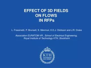
EFFECT OF 3D FIELDS ON FLOWS IN RFPs L. Frassinetti, P. Brunsell, S. Menmuir, K.E.J. Olofsson and J.R. Drake Association EURATOM-VR , School of Electrical Engineering, Royal Institute of Technology KTH, Stockholm. OUTLINE. Experimental tools : - EXTRAP T2R - The feedback system

E N D
EFFECT OF 3D FIELDS ON FLOWS IN RFPs L. Frassinetti, P. Brunsell, S. Menmuir, K.E.J. Olofsson and J.R. Drake Association EURATOM-VR , School of Electrical Engineering, Royal Institute of Technology KTH, Stockholm
OUTLINE • Experimental tools: - EXTRAP T2R - The feedback system - External magnetic perturbations • Plasma flow and Tearing Modes (TM) braking with - non-Resonant Magnetic Perturbations (non-RMP) (m=1, n=-10) - Resonant Magnetic Perturbations (RMP) (m=1, n=-12)(m=1, n=-15) • TM dynamics on short time scale (0.1ms) with RMP and non-RMP • Modelling and viscosity profile estimation
EXTRAP T2R safety factor -12 -12 -10 -13 -14 -15 -15 -16 (m=1 n<-12) are resonant EXTRAP T2R 100 75 50 25 0 EXTRAP T2R TM velocity 20-80 km/s flow (km/s) RFX-mod TM mainly wall locked 0 0.5 1.0 1.5 2.0 Te (keV) • R/a=1.24m/0.183m • Ip < 150kA • tpulse≈ 0.1 s TM velocities: 4x64 local sensors for bq Plasma flow: Passive Doppler spectroscopy for OV, OIV, OIII, OII
active coils sensor coils 1.0 0.8 0.6 0.4 0.2 0.0 1.0 0.8 0.6 0.4 0.2 0.0 Intelligent Shell No Feedback • With the Intelligent Shell: - RWMs - Error fields are suppressed br(mT) br(mT) 0 10 20 30 40 50 60 70 Time (ms) 0 10 20 30 40 50 60 70 Time (ms) (cm) (cm) • The LCFS is much smoother LCFS LCFS THE FEEDBACK SYSTEM The system is composed of: - Sensor coils 4 poloidal x 32 toroidal located inside the shell - Digital controller - Active coils 4 poloidal x 32 toroidal located outside the shell shell tshell≈13.8ms (nominal)
EXTERNAL MAGNETIC PERTURBATION • It is useful to apply only a single external harmonic in order to have an easier interpretation of the results Measured spectrum at the plasma surface 1.0 0.8 0.6 0.4 0.2 0.0 harmonic (1,-12) from 10ms to 30ms amplitude 0.4mT br(mT) 0 10 20 30 40 50 60 70 Time (ms) (cm) 0.15 0.10 0.05 0 -0.05 -0.10 -015 Measured spectrum at t=25ms LCFS at t=25ms
[Frassinetti et al., submitted to NF] 4 3 2 1 0 br1,-12 I1,-12 (A) I1,-12 Measured br spectrum n 0 20 40 60 time (ms) p p/2 0 -p/2 -p time (ms) br1,-12 Applied current spectrum phase (1,-12) I1,-12 n [Olofsson et al., Fus. Eng. Des. 2009] [Olofsson et al., PPCF 2010] [Frassinetti et al., IAEA 2010] 0 20 40 60 time (ms) time (ms) EXTERNAL MAGNETIC PERTURBATION • The feedback needs to: • suppress error fields • suppress RWMs • apply the perturbation • consider the plasma response to the external perturbation The work done by the active coils is not obvious:
WITH PERTURBATION (m,n)=(1,-12) 1.0 0.8 0.6 0.4 0.2 0 br (mT) 60 40 20 0 velocity (km/s) flow TM velocity 0 20 40 60 time (ms) velocity profile (TM) t=20ms t=40ms • with the perturbation: - reduction of the TM velocity - reduction of the plasma flow toroidal velocity (km/s) r/a FLOW AND TM VELOCITY WITH RMP NO PERTURBATION 1.0 0.8 0.6 0.4 0.2 0 br (mT) 60 40 20 0 velocity (km/s) flow TM velocity (1,-12) (1ms smoothed) 0 20 40 60 80 time (ms) • TMs rotate with velocities comparable to the flow
RMP (far from axis) non-RMP 0.10 0.05 0.00 0.10 0.05 0.00 (1,-10) q(r) q(r) (1,-15) 0.0 0.1 0.2 0.3 0.4 0.5 0.6 r/a 0.0 0.1 0.2 0.3 0.4 0.5 0.6 r/a shot 22624 shot 22668 0 -5 -10 -15 -20 -25 0 -5 -10 -15 -20 -25 (1,-15) (1,-10) RMP (far from axis) non-RMP Dv (km/s) Dv (km/s) 0.0 0.1 0.2 0.3 0.4 0.5 0.6 r/a 0.0 0.1 0.2 0.3 0.4 0.5 0.6 r/a • Different RMP harmonicc produce different velocity braking • Maximum braking located at the radius where the RMP harmonic is resonant VELOCITY BRAKING PROFILE RMP (close to axis) 0.10 0.05 0.00 q(r) (1,-12) 0.0 0.1 0.2 0.3 0.4 0.5 0.6 r/a shot 22623 0 -5 -10 -15 -20 -25 (1,-12) RMP (close to axis) Dv (km/s) 0.0 0.1 0.2 0.3 0.4 0.5 0.6 r/a
MAX velocity variation Dv (km/s) non-RMP RMP n (harmonic of external perturbation) ROLE OF THE PERTURBATION HELICITY Set of 13 shots with different harmonic of the perturbation n but same amplitude: brn0.4mT
ROLE OF THE PERTURBATION HELICITY Set of 13 shots with different harmonic of the perturbation n but same amplitude: brn0.4mT OV velocity variation TM velocity variation Dv (km/s) Dv (km/s) non-RMP RMP non-RMP RMP n (harmonic of external perturbation) n (harmonic of external perturbation)
RMP br (mT) velocity (km/s) flow TM velocity (1ms smoothed) 0.1ms TM amplitude (mT) (mT) TM amplitude 0.1ms [Frassinetti, NF 2010] (km/s) (km/s) TM velocity (not smoothed) TM velocity (not smoothed) time (ms) time (ms) • WithRMP clear correlation between velocity and TM amplitude EVOLUTION ON A SHORT TIME SCALE non-RMP br (mT) velocity (km/s) flow TM velocity (1ms smoothed)
EVOLUTION ON A SHORT TIME SCALE Island with RMP LCFS (1,-12) island • Island width: amplification and suppression • Island velocity: acceleration and deceleration depending of relative phase between TM and RMP Rotating TM Static RMP f
RMP n=-12 80 60 40 20 0 t=t0 t=t0+2µs t=t0+4µs t=t0+6µs TM velocity (km/s) n=-12 island 0.0 0.2 0.4 0.6 r/a VELOCITY EVOLUTION WITH RMP br (mT) velocity (km/s) time (ms) velocity (km/s) 0.1ms time (ms) • The island is not simply • slowed down • It has strong • velocity modulations
RMP n=-12 RMP n=-15 80 60 40 20 0 80 60 40 20 0 t=t0 t=t0+2µs t=t0+4µs t=t0+6µs n=-15 island TM velocity (km/s) TM velocity (km/s) t=t0 t=t0+2µs t=t0+4µs t=t0+6µs n=-12 island 0.0 0.2 0.4 0.6 r/a 0.0 0.2 0.4 0.6 r/a velocity variation r/a -10 -5 0 5 10 15 20 time (ms) VELOCITY EVOLUTION WITH RMP br (mT) velocity (km/s) time (ms) velocity (km/s) 0.1ms time (ms) • The island is not simply • slowed down • It has strong • velocity modulations
RMP n=-12 RMP n=-15 80 60 40 20 0 80 60 40 20 0 t=t0 t=t0+2µs t=t0+4µs t=t0+6µs n=-15 island TM velocity (km/s) TM velocity (km/s) t=t0 t=t0+2µs t=t0+4µs t=t0+6µs n=-12 island 0.0 0.2 0.4 0.6 r/a 0.0 0.2 0.4 0.6 r/a velocity variation velocity variation r/a -10 -5 0 5 10 15 20 time (ms) -5 0 5 10 15 20 25 30 time (ms) VELOCITY EVOLUTION WITH RMP br (mT) velocity (km/s) time (ms) velocity (km/s) 0.1ms time (ms) • The island is not simply • slowed down • It has strong • velocity modulations • The velocity perturbation is mainly located • at the island position • But then it “spreads” to • the surrounding plasma [Frassinetti et al., IAEA 2010]
EXPERIMENTAL DATA SIMULATED DATA velocity profile with RMP n=-15 velocity profile with RMP n=-15 r/a r/a time (µs) time (µs) [Frassinetti et al., APS 2010] TORQUE BALANCE EQUATION (RMP) Data are modelled using the torque balance equation. [Fitzpatrick et al. PoP 7, 3610 (2000)] [Guo et al. PoP 9, 4685 (2002)] Reasonable agreement between modelled and experimental data
viscosity profile 10-7 (kg/m∙s) VISCOSITY ESTIMATION (RMP) The viscosity profile is modelled using 3 free parameters exp. data The free parameters are determined by comparing simulated and experimental velocity using a n=-15 RMP. model Viscosity is m10-7kg/(m∙s) This corresponds to a momentum confinement time: tM a2r0/m 1ms RMP n=-15
VISCOSITY ESTIMATION (non-RMP) non-RMP (1,-10) The observed plasma rotation braking is compared with simple empirical model: [R.J. La Haye et al, PoP 9 (2002)2051] tM - momentum confinement time heff- effective frequency Experimental data are well fitted with tM 3ms and heff = 4x10⁶ s-1 br (mT) flow (km/s) [Brunsell et al., EFDA MHD TG meeting 2010]
Dv (km/s) RMP non-RMP n CONCLUSIONS • External magnetic perturbations produce plasma flow and TM braking • RMPs: - The maximum braking is located in the position where the RMP is resonant - The island has phases with amplification-suppression and acceleration-deceleration - The estimated viscosity is approximately 10-7 kg/(m∙s) [tM1ms] • Non-RMPs - The maximum braking is located in the core - The estimated momentum confinement is tM3ms TM velocity variation • What happens if a RMP is applied to RFX-mod? • TMs are wall locked, do we still see a flow braking? • Do we see a transition in the flow braking from RMP to non-RMP? ?