Enhancing Coastal Ocean Predictions with Statistical Data Assimilation Techniques
This study by North Carolina State University focuses on improving the prediction of coastal ocean responses to tropical storms and hurricanes, specifically through advanced data assimilation methods combining observational data with forecasts from the Princeton Ocean Model (POM). With significant investments in coastal areas and rising storm hazards, the research aims to enhance storm surge predictions. The methodology includes using Ensemble Kalman Filtering methods and the initialization of asymmetric wind models to better simulate water level changes during hurricane events, particularly Hurricane Floyd.


Enhancing Coastal Ocean Predictions with Statistical Data Assimilation Techniques
E N D
Presentation Transcript
NC State University Statistical Data Assimilation for Coastal Ocean Prediction Kristen Foley1, Montserrat Fuentes1, Lian Xie2, Shaowu Bao2 North Carolina State University 1Department of Statistics, 2 Department of Marine, Earth and Atmospheric Sciences Motivation The Carolinas has had a tremendous residential and commercial investment in coastal areas during the past 10 years. However rapid development of the coastal region produces a stressed ecosystem and an exponential increase in human and property exposure to storm hazards. Our goal is improve the prediction of the coastal ocean response to tropical storms and hurricanes by using data assimilation techniques to combine available observations (from buoys, ships, satellite, etc.) with the forecasts from the Princeton Ocean Model (POM). Our first goal is to try and improve the prediction of storm surge which is the rise of water caused by tropical cyclone wind and pressure. Model Inputs Ensemble of 10 different input fields for POM for the initial surface water elevation for Sept. 15th hour 03. Model is initialized using both blocking schemes. Below we see the initial fields when the domain is split into 5 independent blocks. • Summary • Storm surge caused by the high speed winds of a hurricane are predicted using a numerical ocean model and observational data from water level stations. • Using Ensemble Kalman Filtering methods we study the impact of dividing the model domain into independent blocks to assist in computation. • Future research includes improving the wind fields used to initialize the model. We also plan to compare these results to the Extended KF as well as more advanced Bayesian Filtering methods. Figure 4:Ensemble of initial surface water elevation (in meters). Data Assimilation Notation Xt(ti)=Xit true (unknown) change of water elevation at time ti. Yio new vector of observations from water level stations. p=5= number of observation sites within the model domain. Xia analysis state vector, best estimate of the unknown state at time ti based on data assimilation methods. Xif output from the Princeton Ocean Model. n=68929=number of grid point locations used by the numerical model. Grid size = 1'longitude by 1'latitude. Princeton Ocean Model The Princeton Ocean Model (POM) is used to simulate the change in water level along the coast of North and South Carolina and Georgia under strong hurricane forcing conditions. In particular a series of wind fields are used to “spin up” the model. Forcing Parameters A symmetric wind model is used to initiate POM based on track information available from NOAA for the center location and central pressure of Floyd on September 15th and 16th. The parameters of the wind model are estimated using nonlinear least squares. We know that hurricane wind fields are typically asymmetric with stronger wind speeds on the right hand side of the storm. As a next step we wish to combine a new asymmetric wind model with a nonstationary multi- variate process model for the E-W and N-S components of the wind vectors. Improving the quality of these initial wind fields is expected to have a significant impact on the prediction of storm surge along the coast. Hurricane Floyd The current case study is Hurricane Floyd which was classified as a hurricane on Sept. 10, 1999 and moved up the Eastern US coast making land- fall near Cape Fear NC early September 16th. Floyd caused the worst short term flooding on record for SE North Carolina and is the deadliest US tropical cyclone since Agnes of 1972. Updated Water Elevation Fields The ensemble of water level fields are updated using the Ensemble Kalman Filter to combine model output and observed values. The EnsKF calculations were based on a block diagonal structure for the forecast error covariance matrix as defined by the blocking shown in Figure 2. (Plots below based on 5 blocks.) Input Fields to initialize model Forcing Parameters Numerical Ocean Model (Princeton Ocean Model) Observations (water level stations, buoys, satellite, etc) Figure 5: Updated ensemble of surface elevation fields for Sept. 15th hr 18. FILTERING METHODS Final Forecast [Hindcast /Nowcast] (storm surge) Forecasting The analysis water elevation fields are updated in the numerical model which is then used to integrate the analysis field forward in time, 1 hour, 3 hours and 6 hours ahead of the updating time. Below we see the effect of the EnsKF step on the model output compared to the observed values for three of the water level stations. The top row shows the results when 3 blocks were used. The next row of graphs shows the results when 5 blocks are used. In general the output based on both blocking schemes is similar but the analysis using fewer blocks appears to better adjust the water level value based on what is observed at each location. Figure 1:General Data Assimilation Framework Figure 3:Estimated wind field based on track of Hurricane Floyd, Sept. 15 hr 03 to Sept.16 hr 03. Wind speed contour in m/s. Blocking of Model Domain The model domain is split into blocks based on the location of the 5 water level stations. Blocks along the coast (shown in gray) are treated as independent. The remaining grid points away for the coast (shown in white) are grouped together as one block and are not used in the data assimilation process. We wish to study the impact of the blocks by comparing the final analysis and forecasting results based on these two blocking schemes. • Ensemble Kalman Filter • The Ensemble Kalman Filter uses a Monte Carlo approach to generate samples of the state vector and carry out an ensemble of data assimilation cycles. This ensemble is then used to estimate the forecast error covariance. • Forecast Step: • Sample Xj(ti-1) ~ N(Xa(ti-1), Pa(ti-1)), j=1,..., K ( K=10) where the initial Xo(t0)=0 and Po(t0) is an exponential spatial covariance with • nugget = .001, partial sill = .036 and range = 107.1 km. • These values were estimated using Maximum Likelihood estimation based on model output using the symmetric wind field to initialize the model compared to output based on a model run initialized by wind field inputs derived from satellite and buoy observations provided by NOAA Hurricane Research Division. • Compute Xjf(ti)=Mj[Xj(ti-1)], j=1,...,K where M[ ] represents the forward integration of the current water level by the Princeton Ocean Model. • Calculate the sample mean and covariance: Xf(ti), Pf(ti) Analysis Step • Perturb the observations at time ti by adding random noise (in this case Gaussian): Yj*(ti)=Yo(ti)+ηj, ηj~N(0,R), j=1,…,K where R is a diagonal matrix. The observation error variance is based on the variance of one second samples reported by each water level station for each hour. Update each member of the forecast sample with the Kalman Filter update to obtain Xaj(ti), j=1,...,K. This now serves as a sample for time ti and the process repeats. The ensemble sample mean and covariance can be used as estimates of the updated state vector and error covariance: Xa(ti), Pa(ti) * observed value used in update step ____observed value - - -model value ____ensemble mean ….. ensemble member ˆ ˆ Figure 2:Two blocking schemes used to generate the spatial covariance of the initial water elevation fields. Observations Observed hourly water levels at each of the 5 water level stations are adjusted for location and tides. These adjusted water levels can be treated as the change in water elevation from an initial value of 0 meters and in this way can be compared to the model output values. Figure 6:Comparison of model output to observed value (top row = 3 blocks; bottom row=5 blocks). Acknowledgments: This research is supported in part by the NSF VIGRE program and by the Carolina Coastal Ocean Observing and Prediction System (Caro-COOPS) program funded by NOAA. Many thanks to Leonard Pietrafesa and Jerry Davis for their continued support.