Download
1 / 42
490 likes | 980 Vues
Analysis of EBSD Data (L17). 27-750, Fall 2009 Texture, Microstructure & Anisotropy, Fall 2009 B. El-Dasher*, A.D. Rollett, G.S. Rohrer , P.N. Kalu. Last revised: 7 th Nov. ‘09. *now with the Lawrence Livermore Natl. Lab. Overview. Understanding the program: Important menus

E N D
Analysis of EBSD Data (L17) 27-750, Fall 2009 Texture, Microstructure & Anisotropy, Fall 2009 B. El-Dasher*, A.D. Rollett, G.S. Rohrer, P.N. Kalu Last revised: 7th Nov. ‘09 *now with the Lawrence Livermore Natl. Lab.
Overview Understanding the program: Important menus Definition of Grains in OIM Partitioning datasets Cleaning up the data: Types Examples of Neighbor correlation Orientation: System Definition Distribution Functions (ODFs) Plotting ODFs
Overview Misorientation: Definitions - Orientation vs. Misorientation Distribution Functions (MDFs) Plotting MDFs Other tools: Plotting Distributions Interactive tools
Navigating the menus There are two menus that access virtually everything: Check the scan stats Creates new partitions Rotate the orientations of each point about sample frame Imports data as partitions Access to routines that cleanup the dataset Cut out scan sections Use this to export text .ang files Check the partition stats & definition Access to menu for: - Maps - Texture calculation - Texture plots • Change the partition properties: • Decide which points to include • Define a “grain” Export grain ID data associated with each point
Grain Definitions OIM defines a set of points to constitute a grain if: - A path exists between any two points (in the set) such that it does not traverse a misorientation angle more than a specified tolerance - The number of points is greater than a specified number Points with a CI less than specified are excluded from statistics Note: Points that are excluded are given a grain ID of 0 (zero) in exported files
Grain Definitions Examples of definitions 3 degrees 15 degrees Note that each color represents 1 grain
Partitioning Datasets Choose which points to include in analysis by setting up selection formula Use to select by individual point attributes Use to select by grain attributes Selection formula is explicitly written here
Data Cleanup • Neighbor Orient. Correlation • Performed on all points in the dataset • For cleanup level n: • Condition 1: Orientation of 6-n nearest neighbors is different than current point (misorientation angle > chosen) • Condition 2: Orientation of 6-n nearest neighbors is the same as each other • If both conditions are met, the point’s orientation is chosen to be a neighbor’s at random • Repeat low cleanup levels (n=3 max) until no more points change for best results Neighbor Phase Correlation - Same as Grain Dilation but instead of using the grain with most number of neighboring points, the phase with the most number of neighboring points is used • Neighbor CI Correlation • Performed only on points with CI less than a given minimum • The orientation and CI of the neighbor with highest CI is assigned to these points • Use when majority of points are high CI, and only a few bad points exist • Grain Dilation: • Acts only on points that do not belong to any grain as defined • A point becomes part of the grain with the most number of surrounding points • Takes the orientation and CI of the neighboring point with highest CI • Use to remove bad points due to pits or at G.Bs • Grain CI Standardization: • Changes the CI of all points within a grain to be that of the highest within each grain • Most useful if a minimum CI criterion is used in analyzing data (prevents low CI points within a grain from being lost) • Output Options: • Overwrite current dataset • Create “cleaned up” dataset as a new dataset • Write the “cleaned up” dataset directly to file
Neighbor Correlation Example No Cleanup Level 0 Note that Higher cleanup levels are iterative (i.e. Level 3= Levels 0,1,2,3) Level 3
Definition of Orientation By definition an orientation is always relative. The OIM uses the sample surface to define the orthogonal reference frame. Quantities are transformed from sample frame to crystal frame e2s e1s j1 F j2 NB: a more comprehensive discussion of reference frames is given later
Orientation Distribution Functions The ODF displays how the measured orientations are distributed in orientation space Two types of distributions can be calculated: • Discrete ODF: • Bin size defines the volume of each element in orientation space (5ox5ox5o) • Fast calculation • Suitable for most texture strengths but not weak textures if the number of grains is small (consider the number of data points per cell required to achieve reasonably low noise) • Continuous ODF: • Generalized Spherical Harmonic Functions: Rank defines the “resolution” of the function • Equivalent to a Fourier transform • Calculation time rises steeply with rank number (32 is an effective maximum) • Time intensive • Mostly appropriate for weaker textures • Some smoothing is inherent
Plotting Orientation Distributions One must select the types of data visualization desired • Inverse Pole Figures are used to illustrate which crystal plane normals are parallel to sample directions (generally RD, TD & ND) • The indices entered represent which sample reference frame plane is being considered: 100, 010 and 001 are typical choices • Multiple planes also need to be entered one at a time • Euler space plot shows the distribution of intensity as a function of the Euler angles • Used to visualize pockets of texture as well as “fiber” textures • Resolution defines how many slices are possible in the plot • Pole figures show the distribution of specific crystal planes w.r.t. sample reference frame • For the generation of more than one PF, they need to be added one at a time.
Types of ODF/Pole Figure/ Inverse PF Plots Choose texture and desired plot type Use to add multiple plots to the same image NB: a more comprehensive discussion of reference frames is given later
Courtesy of N. Bozzolo Preparation of the data for analysis The Average Orientation of the pixels in a grainis given by this equation: Very simple, n’est-ce pas? However, there is a problem... As a consequence of the crystal symmetry, there are several equivalent orientations.This example illustrates the point: i=1,24 RD {111} • 10 000 orientations near to the Brass component: • represented • by a {111} pole figure • and, in the complete Euler space to show the 24 equivalents resulting from application of cubic crystal symmetry Cho J H, Rollett A D and Oh K H (2005) Determination of a mean orientation in electron backscatter diffraction measurements, Metall. Mater. Trans. 36A 3427-38
Parameters for texture analysis max = 5.56 ... 1=0° 1=5° 1=10° 1=15° ... Courtesy of N. Bozzolo
Resolution 32x32x16 Gaussian 3° Lmax 22 Bin Size 5° 16x16x8 3° 22 5° 32x32x16 8° 22 5° max = 5.56 max = 5.37 max = 4.44 Parameters for texture analysis Courtesy of N. Bozzolo Effect of the binning resolution Effect of the width of the Gaussian
Lmax = 34 Lmax = 22 Lmax = 8 Lmax = 5 Lmax = 16 max = 6.36 max = 5.56 max = 5.17 max = 4.04 max = 2.43 Courtesy of N. Bozzolo Effect of the maximum rank in the series expansion, Lmax Resolution 32x32x16 Gaussian 3° Lmax 22 Bin Size 5°
Direct Method max = 5.56 1=5° Courtesy of N. Bozzolo In effect the harmonic method gives some ”smoothing" . Without this, a coarse binning of, say, 10°, produces a very “lumpy” result. Same, with 10°binning : max = 31 !
0.7 1.4 2.0 2.8 4.0 5.6 8.0 11.3 16.0 5.8 at {5 30 15} 6.7 at {0 35 30} 6.6 at {0 35 30} 8.3 at {15 30 30} 7.6 at {0 35 30} Statistical Aspects 0= 4° Texture = distribution of orientations Problem of sampling! 9.0 at {-5 30 40} 8.2 at {0 30 25} 15.5 at {-5 35 50} Triclinic sample symmetry 0= 8° • Number of grains measured • Width of the Gaussian ( and/or Lmax) • Influence of the sample symmetry 6.9 at {-5 35 35} 7.1 at {0 35 25} 7.3 at {345 35 50} 16000 grains 80000 grains 2000 grains 0= 8° Orthorhombic sample symmetry Zirconium, equiaxed Sections thru the OD at constant 1 (Lmax = 34) Gaussienne de 0= 4° Courtesy of N. Bozzolo 7.9 at {0 35 30}
RD (00.1) {10.0} TD ND 0.7 4.0 1.4 5.6 2.0 8.0 2.8 11.3 Courtesy of N. Bozzolo Statistical Aspects Homogeneity/heterogeneity of the specimen... Not just the number of grains must be considered but also their spatial distribution: Single EBSD map (1 mm2) Multiple maps, different locations ( total =1 mm2) equiaxed Ti asymmetry of intensity
j = 0 ° 1 0 0.7 1.4 7.41 2.0 F 2.8 4.0 5.6 8.0 11.3 16.0 90 D > 2D (=11 µm) j 0 60 3496 grains 2 D < D/2 (=2.75 µm) 17.9% surf. 14255 grains 1.7% surf. Global texture Texture – Microstructure Coupling Example : partial texture of populations of grains identified by a grain size criterion (zirconium at the end of recrystallization ) partial texture of the largest grains Partial texture of the smallest grains Important for texture evolution during grain growth: the large grains grow at the expense of the small grains. Since the large grains have a different texture, the overall texture also changes during growth.
Definition of Misorientation Misorientation is an orientation defined with another crystal orientation frame as reference instead of the sample reference frame Thus a misorientation is the axis transformation from one point (crystal orientation) in the dataset to another point z gB y x,y,z are sample reference axes gA is orientation of data point A (reference orientation) w.r.t sample reference gB is orientation of data point B w.r.t. sample reference gA-1 x Misorientation = gBgA-1
Misorientation Distribution Functions Calculating MDFs is very similar to calculating ODFs • Again the function can be either discrete or continuous • Correlated MDF: • Misorientations are calculated only between neighbors • If the misorientation is greater than the grain definition angle, the data point is included • This effectively only plots the misorientations between neighboring points across a G.B. • Uncorrelated MDF: • Misorientations are calculated between all pairs of orientations in dataset • This is the “texture derived” MDF as it effectively is calculated from the ODF • Only effectively used if the sample has weak texture • Texture Reduced: • Requires both Correlated and Uncorrelated MDFs to be calculated for the same plot type • This MDF is simply the Correlated / Uncorrelated values • May be used to amplify any features in the correlated MDF
Plotting MDFs Again, you need to choose what data you want to see Select the Texture dataset Select the plot type (axis/angle ; Rodrigues; Euler) Use to generate plot sections
Charts Charts are easy to use in order to obtain statistical information Increasing bin #
Reconstructed Boundaries • The software includes an analysis of grain boundaries that outputs the information as a (long) list of line segment data. • use of the GB segment analysis is an essential preliminary step before performing the stereological 5-parameter analysis of GBCD. • The data must be on a hexagonal/triangular grid. If you have a map on a square grid, you must convert it to a hexagonal grid. Use the software called OIMTools to do this (freely available fortran program). • Data MUST be on hexagonal grid • Clean up the data to desired level • Choose boundary deviation limit • Generate a map with reconstructed boundaries selected • Export g.b. data into text file • This type of data is required for stereological analysis of 5-parameter grain boundary character
Reference Frames • This next set of slides is devoted to explaining, as best we can, how to relate features observed in EBSD images/maps to the Euler angles. • In general, the Euler frame is not aligned with the x-y axes used to measure locations in the maps. • The TSL and Channel softwares both rotate the image 180° relative to the original physical sample. • Both TLS and Channel softwares use different reference frames for measuring spatial location versus the the Euler angles, which is, of course, extremely confusing.
Zspatial points in to the planeZEuler points out of the plane TSL / OIM Reference Frames TD = yEuler = 010sample xspatial + The purple line indicates a direction, associated with, say, a scratch, or trace of a grain boundary on the specimen. RD = xEuler=100sample Physical specimen:Mounted in the SEM, the tilt axisis parallel to “xspatial” yspatial Image:Note the 180° rotation. ND= zEuler Sample Reference Frame for Orientations/Euler Angles -TD= -yEuler “+” denotes the Origin -RD= -xEuler Crystal Reference Frame: Remember that, to obtain directions and tensor quantities in the crystal frame for each grain (starting from coordinates expressed in the Euler frame), one must use the Euler angles to obtain a transformation matrix (or equivalent). + yspatial xspatial Zspatial Reference Frame for Spatial Coordinates
TSL / OIM Reference Frames for Images Conversion from spatial to Euler and vice versa (TSL only) From Herb Miller’s notes: The axes for the TSL Euler frame are consistent with the RD-TD-ND system in the TSL Technical Manual, but only with respect to maps/images, not the physical specimens. The axes for the HKL system are consistent with Nathalie Bozzolo’s notes and slides. Here, x is in common, but the two y-axes point in opposite directions. Note that the transformation is a 180° rotation about the line x=y Notes: the image, as presented by the TSL software, has the vertical axis inverted in relation to the physical sample, i.e. a 180° rotation.
TSL / OIM Reference Frames: Coordinates in Physical Frame, Conversion to Image • The previous slides make the point that a transformation is required to align spatial coordinates with the Euler frame. • However, there is also a 180° rotation between the physical specimen and the image. Therefore to align physical markings on a specimen with traces and crystals in an image, it is necessary to take either the physical data and rotate it by 180°, or to rotate the crystallographic information. Sample Reference Frame for Orientations ND= zEuler -TD= -ysample • How to measure lines etc. on a physical specimen? • Answer: use the spatial frame as shown on the diagram to the left (which is NOT the normal, mathematical arrangement of axes) and your measured coordinates will be correct in the images, provided you plot them according to the IMAGE spatial frame. The purple line, for example, will appear on the image (e.g. an IPF map) as turned by 180° in the x-y plane. -RD= -xEuler + yspatial xspatial Zspatial
Cartesian Reference Frame for Physical Measurement • How to measure lines etc. on a physical specimen using the standard Cartesian frame with x pointing right, and y pointing up? • Answer: use the Cartesian frame as shown on the diagram to the left (which IS the normal, mathematical arrangement of axes and is NOT the frame used for point coordinates that you find in a .ANG file). Apply the transformation of axes (passive rotation) as specified by the transformation matrix shown and then your measured coordinates will be in the same frame as your Euler angles. This transformation is a +90° rotation about zsample. In this case, the z-axis points out of the plane of the page. xEuler yCartesian yEuler xCartesian
TSL / OIM Reference Frames: Labels in the TSL system The diagram is reproduced from the TSL Technical Manual; the designation of RD, TD and ND is only correct for Euler angles in reference to the plotted maps/images, not the physical specimen = xspatial= yEuler = yspatial= xEuler • What do the labels “RD”, “TD” and “ND” mean in the TSL literature? • The labels should be understood to mean that RD is the x-axis, TD is the y-axis and ND the z-axis, all for Euler angles (but not spatial coordinates). • The labels on the Pole Figures are consistent with the maps/images (but NOT the physical specimen). • The labels on the diagram are consistent with the maps/images, but NOT the physical specimen, as drawn. • The frame in which the spatial coordinates are specified in the datasets is different from the Euler frame (RD-TD-ND) – see the preceding diagrams for information and for how to transform your spatial coordinates into the same frame as the Euler angles, using a 180° rotation about the line x=y.
TSL versus HKL Reference Frames • The two spatial frames are the same, exactly as noted by Changsoo Kim and Herb Miller previously. The figures show images (as opposed to physical specimen). • The Euler angle references frames differ by a rotation of +90° (add 90° to the first Euler angle) going from the TSL to the HKL frames (in terms of an axis transformation, or passive rotation). Vice versa, to pass from the HKL to the TSL frame, one needs a rotation of -90° (subtract 90° from the first Euler angle). • The position of the “sample” axes is critical. The names “RD” and “TD” do not necessarily correspond to the physical “rolling direction” and “transverse direction” because these depend on how the sample was mounted in the microscope. TD=010sample= yEuler TD=010sample= yEuler RD=100sample = xEuler xspatial xspatial + Z (x) + Z (x) RD=100sample= xEuler yspatial yspatial HKL TSL
1 HKL 1 Test of Euler Angle Reference Frames Hexagonal crystal symmetry (no sample symmetry) Euler angles: 17.2°, 14.3°, 0.57° A simple test of the frames used for the Euler angles is to have the softwares plot pole figures for a single orientation with small positive values of the 3 angles. This reveals the position of the crystal x-axis via the sense of rotation imposed by the second Euler angle, F. Clearly, one has to add 90° to 1 to pass from HKL coordinates to TSL coordinates. Note that the CMU TSL is using the x//1120 convention (“X convention”), whereas the Metz Channel/HKL software is using the y//1120 convention (“Y convention”). TSL
The Axis Alignment Issue • The issue with hexagonal materials is the alignment of the Cartesian coordinate system used for calculations with the crystal coordinate system (the Bravais lattice). • In one convention (e.g. popLA, TSL), the x-axis, i.e. [1,0,0], is aligned with the crystal a1 axis, i.e. the [2,-1,-1,0] direction. In this case, the y-axis is aligned with the [0,1,-1,0] direction. • In the other convention, (e.g. HKL, Univ. Metz software), the x-axis, i.e. [1,0,0], is aligned with the crystal [1,0,-1,0] direction. In this case, the y-axis is aligned with the [-1,2,-1,0] direction. • See next page for diagrams. • This is important because texture analysis can lead to an ambiguity as to the alignment of [2,-1,-1,0] versus [1,0,-1,0], with apparent 30° shifts in the data. • Caution: it appears that the axis alignment is a choice that must be made when installing TSL software so determination of which convention is in use must be made on a case-by-case basis. It is fixed to the y-convention in the HKL software. • The main clue that something is wrong in a conversion is that either the 2110 & 1010 pole figures are transposed, or that a peak in the inverse pole figure that should be present at 2110 has shifted over to 1010.
a3 // a2 // x // [100]Cartesian y // [010]Cartesian y // [010]Cartesian a1 // x // [100]Cartesian Diagrams
Euler Angles • To add to the confusion, all of the different Euler angle conventions can, and are used for hexagonal materials. • Recall that Bunge Euler angles make the second rotation about the x-axis, whereas Roe, Matthies and Kocks angles rotate about the y-axis. • Generally speaking there is no problem provided that one stays within a single software analysis system for which the indexing is self-consistent. There are, however, known issues with calculation of inverse pole figures in the popLA package.
Xpix Z1 Ypix top Ypix X1 Xpix Y1 CS1 = raw data format bottom CS0 is modified by the user to align axes however they please. The CTF format always exports in CS0 arrangement. first acquired pixel (Xpix=1,Ypix=1) Euler angle reference frame "Virtual chamber" of HKL software, which is used to define the specimen orientation in the microscope chamber (= how to align frame_0 with frame_1); picture is drawn as if the observer was the camera. Note that the maps are turned by 180° with respect to this picture. - original Euler angles are given in frame_1 (also called CS1) The ctf format is designed to export Euler angle into frame_0 (CS0), which is correct, provided that the specimen orientation is correctly defined. 39
HKL software keeping CS0 (sample frame) aligned with CS1(microscope frame) • relying on what the virtual chamber is showing : Xpix Z1 Ypix top Ypix X1 Xpix Y1 CS1 as shown in the virtual chamber bottom first acquired pixel (Xspatial=1,Yspatial=1) = top left pixel of the resulting map CS1 • but this alignment is not consistent with the axes of the PF plots…or with previous experience with data sets from the HKL software
beta-transformed Ti (from Nathalie Gey, LETAM – now LEM3) (Z0 pointing out) Traces of {10-10} planes Xspatial EBSD map Euler frame Yspatial Xpix, Ypix = spatial frame X0,Y0,Z0 = euler angle frame, supposed to be aligned with X1,Y1,Z1 (µscope frame) Spatial frame Note that a rotation of the PF axes by 180° around Z to recover the frame numbered 3 on the PF plots, would also be consistent with the trace being perpendicular to <10-10>…
Notes on HKL Frames There is a discrepancy in the HKL software between how the frame CS1 (and CS0) is represented in the virtual chamber and how the PF axes are placed The difference is a rotation by 180° around the Z direction (frame numbered 2 versus frame 3) It is not possible to determine which one is correct from the two previous slides Nevertheless, the test maps acquired with LETAM's HKL system and with MRSEC's TSL one did show that the frame number 2 was the correct one