Download
1 / 32
380 likes | 650 Vues
Seismology Part X: Interpretation of Seismograms. Seismogram Interpretation How do we interpret the information we get from a recording of ground motion?. What kinds of information can we extract? How do we figure out what phases we are looking at? These guys look pretty random!.

E N D
Seismology Part X: Interpretation of Seismograms
Seismogram Interpretation How do we interpret the information we get from a recording of ground motion? What kinds of information can we extract? How do we figure out what phases we are looking at? These guys look pretty random!
Until we have a model, we have to look at many seismograms and look for coherent energy.
Here’s another example from an IRIS poster. This is essentially how the first models of the Earth’s interior were generated by Harold Jeffreys and Keith Bullen Harold Jeffreys (1891-1989)
Once we identy phases, we can plot them up on a T-D graph and see if we can match their arrival times with a simple model. It turns out we can explain most of what we see with a very simple crust-mantle-core 1D structure!
The simple 1D model is shown here, along with the basics of seismic phase nomencalture
Local Body Wave Phases • Direct Waves: P & S • Short distance: Pg (granite) • Critically refracted (head): Pn (moho), P* (Conrad; sometimes Pb – basaltic) • Reflected from Moho: PmP (and PmS, etc.)
Basics of Nomencalture Reflected close to source (depth phase): pP, pS, sP, sS Reflected at a distance: PP &SS (and additional multiples) Reflected from the CMB: c, like PcP or ScS Outer Core P wave: K (Kernwellen -> German for Core) Inner Core P wave: I Inner Core S wave: J Reflection at Outer-Inner Core boundary: i (like PKiKP) Ocean wave in SOFAR Channel: T
Paths of P waves in the Earth. Notice the refractions at the CMB that cause a P shadow zone.
Penetration of the Shadow zone by Refractions from the Inner Core
Details of the Current 1D model of the Earth. Note phase transitions in the upper mantle
Interpretation of travel time curves (T vs ) • Locating Earthquakes: • 1. Triangulation • 2. General Inverse problem (below) • Grid search • Tomography: Explaining the • remainder with wavespeed variations
How to model just about anything In general, we can formulate a relationship between model m and observables d as: g(m) = d
we can solve the above by taking a guess mo of m, and expanding g(m) about this guess: Then or Gm = R where G is a matrix containing the partial derivatives. G is an m x n matrix, where m is the number of observations (rows) and n is the number of variables (columns). R is a m x 1 vector or residuals. The idea is to solve the above for m, add it to mo, and then repeat the operation as often as is deemed (statistically) useful.
How to do this? Let’s from the matrix S from G and it’s complex conjugate transpose as: Note that S is a square matrix (N + M) x (N + M) and also S’ = S, which means that there exists an orthogonal set of eigenvectors w and real eigenvalues l such that We solve this eigenvalue problem by noting that non trivial solutions to
will occur only if the determinate of the matrix in the parentheses vanishes: in general there will be (N+M) eigenvalues. Now, each eigenvector w will have N+M components, and it will be useful to consider w as composed of an N dimensional vector v and an M dimensional vector u: Thus, we arrive at the coupled equations:
Note that we can change the sign of and have (-ui, vi) be a solution as well. Thus, there are p pairs of nonzero eigenvalues +-. Let’s suppose there are p pairs of nonzero eigenvalues for the above equations. For the remaining zero eigenvalues, we have Or, in other words, u and v are independent. Now, note that in the non-zero case: GGT and GTG are both Hermitian, so each of V and U forms an orthogonal set of eigenvectors with real eigenvalues. After normalization, we can the write:
VTV = VVT = I UTU = UUT = I Where V is an N x N matrix of the v eigenvectors, and U is an M x M matrix of the u eigenvectors. We say that U spans the data space, and V spans the model space. In the case of zero eigenvalues, we can divide the U and V matrices up into “p” space and “o” space: U = (Up,Uo) V = (Vp,Vo) Because of orthogonality, UpTUp = I VpTVp = I
BUT UpUpT != I VpVpT != I In this case, we write: or, in sum
since VVT = I, we have This is called the Singular Value Decomposition of G, and it shows that we can reconstruct G just using the "p" part. Uo and Vo are "blind spots" not illuminated by G. NB: for overdetermined problems, be can further subdivide U into a U1 and U2 space, where U2 has extra information not required by the problem at hand. This can be very useful as a null operator for some problems.
Since UoTGm = 0 Then the prediction (Gm=d) will have no component in Uo space, only Up space. If the data have some components in Uo space, then there is no way that they can be explained by G! It is thus a source of discrepancy between d and Gm.
The Generalized Inverse Note that if there are no zero singular values, then we can write down the inverse of G immediately as: G-1 = V-1UT Since G-1G = V-1UT UVT = V-1VT = VVT = I In the case of zero singular values, we can try using the p space only, in which case we have the generalized inverse operator: Gg-1 = Vpp-1UpT Let's see what happens when we apply this
Suppose that there is a Uo space but no Vo space. In this case • GTG = VppUpTUppVpT = Vpp2VpT • has an exact inverse: • (GTG)-1 = Vpp-2VpT • Then we can write: • GTGm = GTd • and • m = (GTG)-1 GTd = Vpp-2VpTVppUpTd • = Vpp-1UpTd = Gg-1d
Note that the generalized inverse gives the least squares solution, defined as the minimum of the squares of the residuals: min|d - Gm|2 Let mg = Gg-1d. Then d - G mg = d - UppVpTVpp-1UpTd = d - UpUpTd Thus UpT(d - G mg) = UpT(d - UpUpTd) = UpTd - UpTd = 0 Which means that there is no component of the residual vector in Up space.
Also, UoT G mg = 0 And so there is no component of the predicted data in Uo space. Imagine the total data space spanned by Uo and Up. The generalized inverse explains all the data that project onto Up, and the residual (d - Gmg) projects onto Uo. What if there is not Uo but Vo space exists? Let's try our mg solution again and see what happens. mg = Gg-1d so Gmg = GGg-1d = UppVpTVpp-1UpTd = UpUpTd = d
So, the solution mg will satisfy d with a model restricted to Vp space. We are free to add on any components of Vo space we like to mg to generate a model m - these will have no effect on the fit to the data. Note however that any such addition will mean a larger net change in m. Thus mg is our minimum step solution out of all possible solutions (cf. Occam's razor!). Finally, when there are both Vo and Uo spaces, the generalized inverse operator will both minimize the model step and the residual. Pretty good, eh?
Resolution and Error Let's compare the "real" solution m to our generalized inverse estimate of it: mg. Recall that mg = Gg-1d Gm = d So mg = Gg-1Gm = Vpp-1UpTUppVpTm = VpVpTm Thus, if there is no Vo space, VpVpT = I and mg and m are the same. In the event of Vo space then mg will be a smoothed version of m. We call the product VpVpT the Model Resolution Matrix.
How about in data space? In this case, we compare the actual data "d" with our predicted data dg: mg = Gg-1d dg = Gmg= GGg-1d = UppVpTVpp-1UpTd = UpUpTd Thus, in the absence of Uo space, the prediction matches the observed. If Uo exists, then dg is a weighted average of d and a discrepancy exists. In this case, we say that parts of d cannot be fit with the model; only certain combinations of d can be fit.
Finally, we can estimate how data uncertainties translate into model uncertainties: mg = Gg-1d We write the covariance of these terms as: mgmgT> = Gg-1<ddT> GgT-1 If all the uncertainties in d are statistically independant and equal to a constant variance d2, then mgmgT> = d2Gg-1GgT-1 =d2Vpp-1UpTUpp-1VpT =d2Vpp-2VpT
Note from above that (GTG)-1 = Vpp-2VpT and so mgmgT> = d2(GTG)-1 Note that the covariance goes up as the singular values get small, so including the associated eigenvectors could be very unstable. There are a couple of ways around this. One is just not to use them (i.e., enforce a cutoff below which a singular value is defined to be zero). The other is damping. To talk about damping quantitatively we need to do some more statistics.