Stanford Linear Accelerator Center

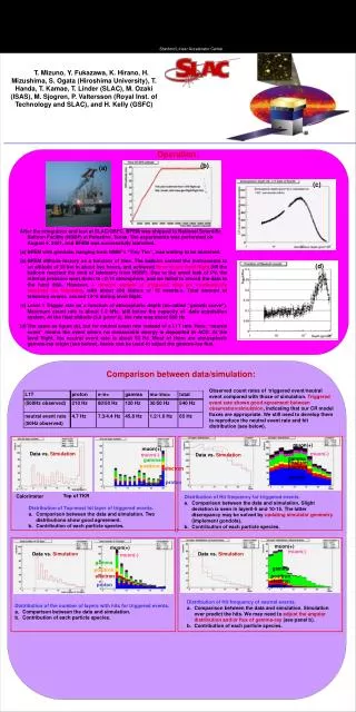
1. Stanford Linear Accelerator Center T. Mizuno, Y. Fukazawa, K. Hirano, H. Mizushima, S. Ogata (Hiroshima University), T. Handa, T. Kamae, T. Linder (SLAC), M. Ozaki (ISAS), M. Sjogren, P. Valtersson (Royal Inst. of Technology and SLAC), and H. Kelly (GSFC) Operation: (b) (a) (c) • After the integration and test at SLAC/GSFC, BFEM was shipped to National Scientific Balloon Facility (NSBF) at Palestine, Texas. The experiments was performed on August 4, 2001, and BFEM was successfully launched. • BFEM with gondola, hanging from NSBF’s “Tiny Tim”, was waiting to be launched. • BFEM altitude history as a function of time. The balloon carried the instruments to an altitude of 38 km in about two hours, and achieved three hours level flight (till the balloon reached the limit of telemetry from NSBF). Due to the small leak of PV, the internal pressure went down to ~0.14 atmosphere, and we failed to record the data to the hard disk. However, a random sample of triggered data are continuously obtained via telemetry, with about 200 kbits/s or 12 events/s. Total amount of telemetry events exceed 10^5 during level flight. • Level 1 Trigger rate as a function of atmospheric depth (so-called “growth curve”). Maximum count rate is about 1.2 kHz, still below the capacity of data acquisition system. At the float altitude (3.8 g/cm^2), the rate was about 500 Hz. • The same as figure (b), but for neutral event rate instead of a L1T rate. Here, “neutral event” means the event where no measurable energy is deposited in ACD. At the level flight, the neutral event rate is about 50 Hz. Most of them are atmospheric gamma-ray origin (see below), hence can be used to adjust the gamma-ray flux. (d) O Comparison between data/simulation: Observed count rates of triggered event/neutral event compared with those of simulation. Triggered event rate shows good agreement between observation/simulation, indicating that our CR model fluxes are appropriate. We still need to develop them to reproduce the neutral event rate and hit distribution (see below). muon(+) muon(+) Data vs. Simulation muon(-) muon(-) Data vs. Simulation gamma gamma positron positron electron electron proton proton Top of TKR Calorimeter • Distribution of Hit frequency for triggered events. • Comparison between the data and simulation. Slight deviation is seen in layer0-5 and 10-15. The latter discrepancy may be solved by updating simulator geometry (implement gondola). • Contribution of each particle species. • Distribution of Top-most hit layer of triggered events. • Comparison between the data and simulation. Two distributions show good agreement. • Contribution of each particle species. muon(+) muon(+) muon(-) Data vs. Simulation Data vs. Simulation muon(-) gamma gamma positron electron positron electron proton proton • Distribution of Hit frequency of neutral events. • Comparison between the data and simulation. Simulation over predict the hits. We may need to adjust the angular distribution and/or flux of gamma-ray (see panel b). • Contribution of each particle species. • Distribution of the number of layers with hits for triggered events. • Comparison between the data and simulation. • Contribution of each particle species.