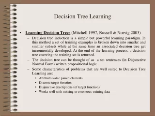
CS 9633 Machine Learning Decision Tree Learning

1. CS 9633 Machine LearningDecision Tree Learning References: Machine Learning by Tom Mitchell, 1997, Chapter 3 Artificial Intelligence: A Modern Approach, by Russell and Norvig, Second Edition, 2003, pages C4.5: Programs for Machine Learning, by J. Ross Quinlin, 1993. Computer Science Department CS 9633 KDD

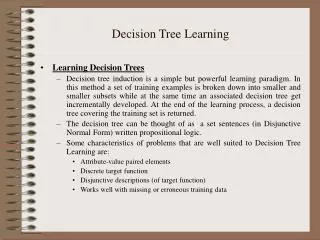
2. Decision Tree Learning • Approximation of discrete-valued target functions • Learned function is represented as a decision tree. • Trees can also be translated to if-then rules Computer Science Department CS 9633 KDD

3. Decision Tree Representation • Classify instances by sorting them down a tree • Proceed from the root to a leaf • Make decisions at each node based on a test on a single attribute of the instance • The classification is associated with the leaf node Computer Science Department CS 9633 KDD

4. Outlook Sunny Overcast Rain Humidity Wind Yes High Normal Strong Weak No Yes No Yes <Outlook = Sunny, Temp = Hot, Humidity = Normal, Wind = Weak>

5. Representation • Disjunction of conjunctions of constraints on attribute values • Each path from the root to a leaf is a conjunction of attribute tests • The tree is a disjunction of these conjunctions Computer Science Department CS 9633 KDD

6. Appropriate Problems • Instances are represented by attribute-value pairs • The target function has discrete output values • Disjunctive descriptions are required • The training data may contain errors • The training data may contain missing attribute values Computer Science Department CS 9633 KDD

7. Basic Learning Algorithm • Top-down greedy search through space of possible decision trees • Exemplified by ID3 and its successor C4.5 • At each stage, we decide which attribute should be tested at a node. • Evaluate nodes using a statistical test. • No backtracking Computer Science Department CS 9633 KDD

8. ID3(Examples, Target_attribute, Attributes) • Create a Root node for the tree • If all examples are positive, return the single node tree Root, with label + • If all examples are negative, return the single node tree Root, with label – • If Attributes is empty, return the single-node tree Root, with label = most common value of Target_Attribute in Examples • Otherwise Begin • A  the number of attribute that best classifies Examples • The decision attribute for Root  A • For each possible value, vi for A • Add a new tree branch below Root corresponding to the test A = vi • Let Examplesvi be the subset of Examples that have value vi for A • If Examples is Empty Then • Below this new branch add a leaf node • Else • Below this new branch add the subtree • ID3(Examplesvi, Target_attribute, Attributes – {A}) • End • Return Root

9. Selecting the “Best” Attribute • Need a good quantitative measure • Information Gain • Statistical property • Measures how well an attribute separates the training examples according to target classification • Based on entropy measure Computer Science Department CS 9633 KDD

10. Entropy Measure Homogeneity • Entropy characterizes the impurity of an arbitrary collection of examples. • For two class problem (positive and negative) • Given a collection S containing + and – examples, the entropy of S relative to this boolean classification is: Computer Science Department CS 9633 KDD

11. Examples • Suppose S contains 4 positive examples and 60 negative examples Entropy(4+,60-)= • Suppose S contains 32 positive examples and 32 negative examples Entropy(32+,32-)= • Suppose S contains 64 positive examples and 0 negative examples Entropy(64+,0-)= Computer Science Department CS 9633 KDD

12. General Case Computer Science Department CS 9633 KDD

13. From Entropy to Information Gain • Information gain measures the expected reduction in entropy caused by partitioning the examples according to this attribute Computer Science Department CS 9633 KDD

15. S: [(G,4)(D,5)(P,6)] E = Marital Status Debt Income Low Medium High Low Medium High Unmarried Married

16. Hypothesis Space Search • Hypothesis space: Set of possible decision trees • Simple to complex hill-climbing • Evaluation function for hill-climbing is information gain Computer Science Department CS 9633 KDD

17. Capabilities and Limitations • Hypothesis space is complete space of finite discrete-valued functions relative to the available attributes. • Single hypothesis is maintained • No backtracking in pure form of ID3 • Uses all training examples at each step • Decision based on statistics of all training examples • Makes learning less susceptible to noise Computer Science Department CS 9633 KDD

18. Inductive Bias • Hypothesis bias • Search bias • Shorter trees are preferred over longer ones • Trees with attributes with the highest information gain at the top are preferred Computer Science Department CS 9633 KDD

19. Why Prefer Short Hypotheses? • Occam’s razor: Prefer the simplest hypothesis that fits the data • Is it justified? • Commonly used in science • There are a smaller number of small hypothesis than larger ones • But some large hypotheses are also rare • Description length influences size of hypothesis • Evolutionary argument Computer Science Department CS 9633 KDD

20. Overfitting • Definition: Given a hypothesis space H, a hypothesis h H is said to overfit the training data if there exists some alternative hypothesis h’ over the training examples, but h’ has a smaller error than h over the entire distribution of instances. Computer Science Department CS 9633 KDD

21. Avoiding Overfitting • Stop growing the tree earlier, before it reaches the point where it perfectly classifies the training data • Allow the tree to overfit the data, and then post-prune the tree Computer Science Department CS 9633 KDD

22. Criterion for Correct Final Tree Size • Use a separate set of examples (test set) to evaluate the utility of post-pruning • Use all available data for training, but apply a statistical test to estimate whether expanding (or pruning) is likely to produce improvement. (chi-square test used by Quinlan at first—later abandoned in favor of post-pruning) • Use explicit measure of the complexity for encoding the training examples and the decision tree, halting growth of the tree when this encoding size is minimized (Minimum Description Length principle). Computer Science Department CS 9633 KDD

23. Two types of pruning • Reduced error pruning • Rule post-pruning Computer Science Department CS 9633 KDD

24. Reduced Error Pruning • Decision nodes are pruned from final tree • Pruning a node consists of • Remove sub-tree rooted at the node • Make it a leaf node • Assign most common classification of the training examples associated with the node • Remove nodes only if the resulting pruned tree performs no worse than the original tree over the validation set. • Pruning continues until it is harmful Computer Science Department CS 9633 KDD

25. Rule Post-Pruning • Infer the decision tree from the training set—allow overfitting • Convert tree into equivalent set of rules • Prune each rule by removing preconditions that result in improving its estimated accuracy • Sort the pruned rules by estimated accuracy and consider them in order when classifying Computer Science Department CS 9633 KDD

26. Outlook Sunny Overcast Rain Humidity Wind Yes High Normal Strong Weak No Yes No Yes If (Outlook = Sunny)  ( Humidity = High) Then (PlayTennis = No)

27. Why convert the decision tree to rules before pruning? • Allows distinguishing among the different contexts in which a decision node is used • Removes the distinction between attribute tests near the root and those that occur near leaves • Enhances readability Computer Science Department CS 9633 KDD

28. Continuous Valued Attributes For a continuous variable A, establish a new Boolean variable Ac that tests if the value of A is less than c A < c How do select a value for the threshold c? Computer Science Department CS 9633 KDD

29. Identification of c • Sort instances by continuous value • Find boundaries where the target classification changes • Generate candidate thresholds between boundary • Evaluate the information gain of the different thresholds Computer Science Department CS 9633 KDD

30. Alternative methods for selecting attributes • Information gain has natural bias for attributes with many values • Can result in selecting an attribute that works very well with training data but does not generalize • Many alternative measures have been used • Gain ratio (Quinlan 1986) Computer Science Department CS 9633 KDD

31. Missing Attribute Values • Suppose we have instance <x1, c(x1)> at a node (among other instances) • We want to find the gain if we split using attribute A and A(x1) is missing. • What should we do? Computer Science Department CS 9633 KDD

32. 2 simple approaches • Assign the missing attribute the most common value among the examples at node n • Assign the missing attribute the most common value among the examples at node n with classification c(x) Node A <blue,…,yes> <red,…, no> <blue,…, yes> <?,…,no> Computer Science Department CS 9633 KDD

33. More complex procedure • Assign a probability to each of the possible values of A based on frequencies of values of A at node n. • In previous example, probabilities would be 0.33 red and 0.67 blue. Distribute fractional instances down the tree and use fractional values to compute information gain. • Can also use these fractional values to compute information gain • This is the method used by Quinlan Computer Science Department CS 9633 KDD

34. Attributes with different costs • Often occurs in diagnostic settings • Introduce a cost term into the attribute selection measure • Approaches • Divide Gain by the cost of the attribute • Tan and Schlimmer: Gain2(S,A)/Cost(A) • Nunez: (2Gain(S,A)-1)/(Cost(A) + 1)w Computer Science Department CS 9633 KDD