Download
1 / 39
390 likes | 418 Vues
Explore the safe design of buildings for dealing with hydrogen leaks, emphasizing the effectiveness of passive ventilation systems. Includes parametric analyses, CFD modeling, and thermal effects.

E N D
Analysis of Buoyancy-Driven Ventilation of Hydrogen from Buildings C. Dennis Barley, Keith Gawlik, Jim Ohi, Russell Hewett National Renewable Laboratory U.S. DOE Hydrogen Safety, Codes & Standards Program Presented at 2nd ICHS, San Sebastián, Spain September 11, 2007
Scope of Work Safe building design Vehicle leak in residential garage Continual slow leak Passive, buoyancy-driven ventilation (vs. mechanical) Steady-state concentration of H2 vs. vent size
Prior Work Modeling and testing with H2 and He Transient H2 cloud formation __________ Swain et al. (1996, 2001, 2003, 2005, 2007) Breitung et al. (2001) Papanikolaou and Venetsanos (2005)
Our Focus / New Findings Slow continual leaks Steady-state concentration of H2 Algebraic equation for vent sizing Significant thermal effect (high outdoor temp)
Range of “Slow” Leakage Rates Low end: 1.4 L/min per SAE J2578 (vehicle manufacture quality control) High end: 566 L/min automatic shutdown (per Parsons Brinkerhoff for CaFCP) Consider: Collision damage or faulty maintenance Parametric CFD modeling: 5.9 to 82 L/min (12 hr to 7 days/5 kg)
Methods of Analysis CFD modeling (FLUENT) Simplified, 1-D, steady-state, algebraic analysis
Volume of garage is 146 m3 Volume of 5 kg of H2 is 60 m3 41% mixture is possible Well within flammable range
Sample CFD Model Result CFD modeling used to study H2 cloud. Half of garage is shown. Leak rate is 5 kg/24 hours (41.5 L/min). Vent sizes 790 cm2. Elapsed time = 83 min. Full scale is 4% H2 by volume.
Sample CFD Model Result H2 concentration at top vent increases monotonically and reaches a steady value in about 90 minutes. A flammable mixture does not occur in this case.
Simulation Setup • FLUENT version 6.3 • Poly mesh for computational economy • Grid density study showed solution invariant at approx. 40,000 cells (Avg. ~1.8 L/cell) • High mesh density near inlet, outlet, gas leak • Laminar flow model used (more conservative than turbulent models) • No diffusion across vents at model boundary
Simulation Setup • Hydrogen concentration at outlet monitored to determine steady state • 5 kg discharge times from 12 hours to 1 week • Low speed leak from 8-cm-diameter sphere • Leak ~1 m above floor, one model near ceiling • Vent sizes and height varied
Concept of 1-D Model Typical H2 stratification determined by CFD model (steady-state condition)
1-D Parametric Analysis Pressure Loop / Buoyancy ΔP1-2 + ΔP2-3 + ΔP3-4 + ΔP4-1 = 0 ΔP1-2 + ΔP3-4 = g h ρair cavg (1-δ) P = Total pressure h = Height between vents c = Concentration of H2, by volume ρ = Density g = Acceleration of gravity δ = Density of H2 / density of air
1-D Parametric Analysis Vent Flow vs. Pressure Q = Volumetric flow rateA = Vent areaD = Discharge coefficient (Similar at bottom vent)
1-D Parametric Analysis Steady-State Mass Balances QT cT = SQ = Volumetric flow rate cT = H2 concentration at top vent, by volume S = Volumetric H2 source rate
1-D Parametric Analysis Isothermal Vent-Sizing Equation: where: F = Vent sizing factor, dimensionless A = Vent area (top = bottom), m2 CT = H2 concentration at top vent, by volume (0-1) D = Vent discharge coefficient (0-1) S = Source rate of H2 (leak rate), m3/s g = Acceleration of gravity = 9.81 m/s2 h = Height between vents, mm δ = Ratio of densities of H2/Air = 0.0717 φ = Stratification factor = CT/Cavg (Cavg = average over height)
Comparison of Models Curves illustrate isothermal vent-sizing equation. Points 1-7 are CFD results.
Ranges of Parameters Stratification factor (φ): 1.52 to 1.88 Apparent discharge coefficient (D*): 0.903 to 0.965 D* higher than typical D (0.60 to 0.70) D* includes momentum effects Further study needed (experimental)
Reverse Thermocirculation When outdoor temperature is higher than indoor (garage) temperature, thermal circulation opposes H2-buoyancy-driven circulation.
Thermal Case Study Leak rate = 5 kg/12 hours. Vent size = 1,580 cm2. Tamb-Tcond = 20°C. Elapsed time = 3.3 min. Full scale = 4% H2 by volume.
Thermal Case Study Leak rate = 5 kg/12 hours. Vent size = 1,580 cm2. Tamb-Tcond = 20°C. Elapsed time = 11.7 min. Full scale = 4% H2 by volume.
Thermal Case Study Leak rate = 5 kg/12 hours. Vent size = 1,580 cm2. Tamb-Tcond = 20°C. Elapsed time = 15 min. Full scale = 4% H2 by volume.
Thermal Case Study Leak rate = 5 kg/12 hours. Vent size = 1,580 cm2. Tamb-Tcond = 20°C. Elapsed time = 33 min. Full scale = 4% H2 by volume.
Thermal Case Study Leak rate = 5 kg/12 hours. Vent size = 1,580 cm2. Tamb-Tcond = 20°C. Elapsed time = 2.8 hr (steady state). Full scale = 4% H2 by volume.
Thermal Case Study Leak rate = 5 kg/12 hours. Vent size = 1,580 cm2. Tamb-Tcond = 20°C.
A Perfect StormExtreme thermal scenario Garage strongly coupled to house & ground Garage weakly coupled to ambient Hot day, cool ground, low A/C setpoint Small vents—sized for 2% H2 max with 1-D model
A Perfect Storm Heartland Homes, Pittsburgh, PA
A Perfect StormAmbient conditions modeled • Ambient temp. = 40.6°C (Approx. max. in Denver) • Ground temp = 10°C (Denver, mid-April) • A/C setpoint = 21.1°C (Rather low)
Reverse Flow ScenarioH2 exiting through bottom vent Case 9. Leak rate = 5 kg/7 days. Vent size = 494 cm2. Elapsed time = 31 hr (steady state). Full scale = 1.5% H2 by volume.
A Perfect StormResults Case 8 (1-day leak): Vents from top, 2.3% max Case 9 (7-day leak): Vents from bottom, 1.0% max Case 10 (3-day leak): Vents from top, 4.8% max
A Perfect StormWorst thermal case we modeled Case 10. Leak rate = 5 kg/3 days. Vent size = 405 cm2.
Conclusions 1. The leakage rates that will occur and their frequencies are unknown. Further study of leakage rates is needed to put parametric results into perspective. 2. Our CFD model has not yet been validated against experimental data. • Uncertainty in results • Future work
3. The 1-D model ignores thermal effects, but otherwise provides a safe-side estimate of H2 concentration by ignoring momentum effects (pending model validation). 4. Indicated vent sizes would cause very low garage temperatures in cold climates, for leak rates of roughly 6 L/min and higher (leak-down in 1 week or less). Conclusions
5. Reverse thermocirculation: Can occur in nearly any climate The worst case we modeled increased the expected H2 concentration from 2% to 5%. This is a significant risk factor, Likelihood of occurrence may be low, judging by the lengths we went to in order to identify a significant example. Conclusions
6. Mechanical ventilation is alternative approach to safety. H2-sensing fan controller is recommended. Research is needed to develop a control system that is sufficiently reliable and economical for residential use. Conclusions