Download
1 / 27
270 likes | 274 Vues
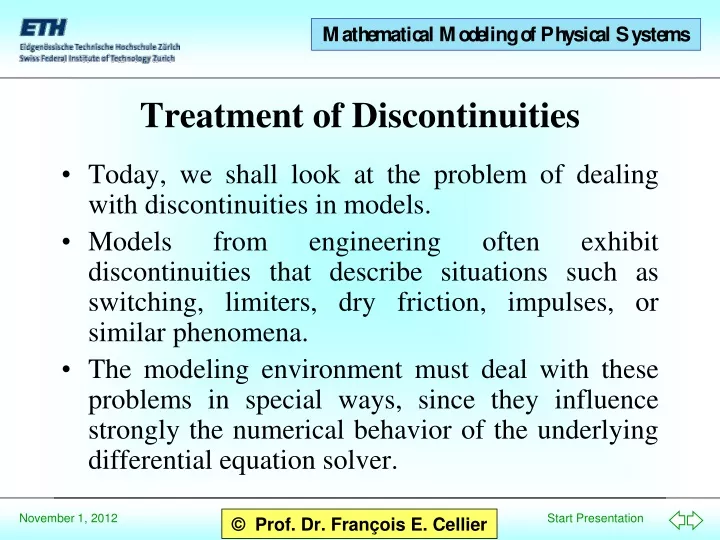
Today, we shall look at the problem of dealing with discontinuities in models. Models from engineering often exhibit discontinuities that describe situations such as switching, limiters, dry friction, impulses, or similar phenomena.

E N D
Today, we shall look at the problem of dealing with discontinuities in models. Models from engineering often exhibit discontinuities that describe situations such as switching, limiters, dry friction, impulses, or similar phenomena. The modeling environment must deal with these problems in special ways, since they influence strongly the numerical behavior of the underlying differential equation solver. Treatment of Discontinuities
Numerical differential equation solvers Discontinuities in state equations Integration across discontinuities State events Event handling Multi-valued functions The electrical switch The ideal diode Friction Table of Contents
Most of the differential equation solvers that are currently on the market operate on polynomial extrapolation. The value of a state variable x at time t+h, where h is the current integration step size, is approximated by fitting a polynomial of nth order through known supporting values of x and dx/dt at the current time t as well as at past instances of time. The value of the extrapolation polynomial at time t+h represents the approximated solution of the differential equation. In the case of implicit integration algorithms, the state derivative at time t+h is also used as a supporting value. Numerical Differential Equation Solvers
· x(t+h) x(t) + h · x(t) · x(t+h) x(t) + h · x(t+h) Examples Explicit Euler Integration Algorithm of 1st Order: Implicit Euler Integration Algorithm of 1st Order:
Polynomials are always continuous and continuously differentiable functions. Therefore, when the state equations of the system: exhibit a discontinuity, the polynomial extrapolation is a very poor approximation of reality. Consequently, integration algorithms with a fixed step size exhibit a large integration error, whereas integration algorithms with a variable step size reduce the step size dramatically in the vicinity of a discontinuity. · x(t) = f(x(t),t) Discontinuities in State Equations
An integration algorithm of variable step size reduces the step size at every discontinuity. After passing the discontinuity, the step size is only slowly enlarged again, as the integration algorithm cannot distinguish between a discontinuity on one hand and a point of large local stiffness (with a large absolute value of the derivative) on the other. Discontinuities The step size is constantly too small. Thus, the integration algorithm is at least highly inefficient, if not even inaccurate. Integration Across Discontinuities h t
These problems can be avoided by telling the integration algorithm explicitly, when and where discontinuities are contained in the model description. 3 1 2 f(x) fp f = fm xm a f = m·x x xp f = fp fm m = tg(a) f = ifx < xm then fm else if x < xp then m*x elsefp ; The State Event Example:Limiter Function
Iteration x xp Threshold t h h f(x) fp Model switching h x xp xm a x xp t t h fm Step size reduction during process of iteration Event Event Handling I
h t h Step size as function of time without event handling Step size as function of time with event handling t Event Handling II
In Modelica, discontinuities are represented as if-statements. In the process of translation, these statements are transformed into correct event descriptions (sets of models with switching conditions). The modeler does not need to concern him- or herself with the mechanisms of event descriptions. These are hidden behind the if-statements. f = ifx < xm then fm else if x < xp then m*x elsefp ; Representation of Discontinuities
The modeler needs to take into account that the discontinuous solution is temporarily left during iteration. may be dangerous, since absDpcan becometemporarily negative. solves this problem. Dp = p1 – p2 ; absDp = ifDp > 0 thenDp else –Dp ; q = sqrt(absDp) ; q = | Dp | Dp = p1 – p2 ; absDp =noEvent(ifDp > 0 thenDp else –Dp ) ; q = sqrt(absDp) ; Problems
The noEvent construct has the effect that if-statements or Boolean expressions, which normally would be translated into simulation code containing correct event handling instructions, are handed over to the integration algorithm untouched. Thereby, management of the simulation across these discontinuities is left to the step size control of the numerical Integration algorithm. Dp = p1 – p2 ; absDp =noEvent(ifDp > 0 thenDp else –Dp ) ; q = sqrt(absDp) ; The “noEvent” Construct
The language constructs that have been introduced so far don’t suffice to describe multi-valued functions, such as the dry hysteresis function shown below. When xbecomes greater than xp, f must be switched from fm to fp. When xbecomes smaller than xm, f must be switched from fp to fm. f(x) fp x xm xp fm Multi-valued Functions I
becomes larger f(x) fp when initial() then reinit(f, fp); end when; when x > xp or x < xm then f = if x > 0 then fp else fm; end when; x xm xp Executed at the beginning of the simulation. } fm These statements are only executed, when either xbecomes larger thanxp,or when xbecomes smaller thanxm. is larger Multi-valued Functions II
i u 0 = ifopenthenielse u ; The Electrical Switch I When the switch is open, the current is i=0. When the switch is closed, the voltage is u=0. The if-statement in Modelica is a-causal. It is being sorted together with all other statements.
0 = s · i + ( 1 – s ) · u Switch open: Sf f = 0 e s Sw The causality of the switch element is a function of the value of the control signal s. Switch closed: f e = 0 Se The Electrical Switch II Possible Implementation: Switch open: s = 1 Switch closed: s = 0
When u < 0, the switch is open. No current flows through. i Switch closed i u u When u > 0, the switch is closed. Current may flow. The ideal diode behaves like a short circuit. Switch open f D open = u <0; 0 = ifopenthenielse u ; e The Ideal Diode I
Since current flowing through a diode cannot simply be interrupted, it is necessary to slightly modify the diode model. The variable open must be declared as Boolean. The value to the right of the Boolean expression is assigned to it. open = u <= 0and noti > 0; 0 = ifopenthenielse u ; The Ideal Diode II
More complex phenomena, such as friction characteristics, must be carefully analyzed case by case. The approach is discussed here by means of the friction example. fB R0 Rm Viscous friction v Dry friction -Rm -R0 The Friction Characteristic I When v 0 , the friction force is a function of the velocity. When v = 0 , the friction force is computed such that the velocity remains 0.
We distinguish between five situations: Sticking: The friction force compensates the sum of all forces attached, except if |Sf | > R0 . v = 0 a = 0 Moving forward: v > 0 The friction force is computed as: fB = Rv · v + Rm. Moving backward: v < 0 The friction force is computed as: fB = Rv·v -Rm. Beginning of forward motion: v = 0 a > 0 The friction force is computed as: fB = Rm. Beginning of backward motion: v = 0 a < 0 The friction force is computed as: fB =-Rm. The Friction Characteristic II
The set of events can be described by a state transition diagram. Start v < 0 v > 0 v = 0 Sf < -R0 Sf > +R0 Backward acceleration (a < 0) Forward acceleration (a > 0) Sticking (a = 0) Backward motion (v < 0) Forward motion (v > 0) a 0 and not v < 0 a 0 and not v > 0 v 0 v 0 v < 0 v > 0 The State Transition Diagram
The Friction Model I model Friction; parameter Real R0, Rm, Rv; parameter Boolean ic=false; Real fB, fc; Boolean Sticking (final start = ic); Boolean Forward (final start = ic), Backward (final start = ic); Boolean StartFor (final start = ic), StartBack (final start = ic); fB = if Forward then Rv*v + Rm else if Backward then Rv*v - Rm else if StartFor then Rm else if StartBack then -Rm else fc; 0 = if Sticking or initial() then a else fc;
when Sticking and not initial() then reinit(v,0); end when; Forward = initial() and v > 0or pre(StartFor)and v > 0or pre(Forward) and not v <= 0; Backward = initial() and v < 0or pre(StartBack)and v < 0or pre(Backward) and not v >= 0; The Friction Model II
StartFor = pre(Sticking) and fc > R0or pre(StartFor)and not (v > 0or a <= 0and not v > 0); StartBack = pre(Sticking) and fc < -R0or pre(StartBack)and not (v < 0or a >= 0and not v < 0); Sticking = not (Forward or Backward or StartFor or StartBack); end Friction; The Friction Model III
Cellier, F.E. (1979), Combined Continuous/Discrete System Simulation by Use of Digital Computers: Techniques and Tools, PhD Dissertation, Swiss Federal Institute of Technology, ETH Zürich, Switzerland. Elmqvist, H., F.E. Cellier, and M. Otter (1993), “Object-oriented modeling of hybrid systems,” Proc. ESS'93, SCS European Simulation Symposium, Delft, The Netherlands, pp.xxxi-xli. Cellier, F.E., M. Otter, and H. Elmqvist (1995), “Bond graph modeling of variable structure systems,” Proc. ICBGM'95, 2nd SCS Intl. Conf. on Bond Graph Modeling and Simulation, Las Vegas, NV, pp. 49-55. References I
Elmqvist, H., F.E. Cellier, and M. Otter (1994), “Object-oriented modeling of power-electronic circuits using Dymola,” Proc. CISS'94, First Joint Conference of International Simulation Societies, Zurich, Switzerland, pp. 156-161. Glaser, J.S., F.E. Cellier, and A.F. Witulski (1995), “Object-oriented switching power converter modeling using Dymola with event-handling,” Proc. OOS'95, SCS Object-Oriented Simulation Conference, Las Vegas, NV, pp. 141-146. References II