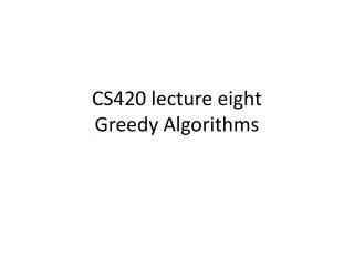
CS420 lecture eight Greedy Algorithms
CS420 lecture eight Greedy Algorithms. Going from A to G. Starting with a full tank, we can drive 350 miles before we need to gas up, minimize the number of times we need to stop at a gas station A B C D E F G

CS420 lecture eight Greedy Algorithms
E N D
Presentation Transcript
Going from A to G • Starting with a full tank, we can drive 350 miles before we need to gas up, minimize the number of times we need to stop at a gas station A B C D E F G 0 250 300 600 850 900 1100
Going from A to G • We can drive 350 miles before we need to gas up, minimize the number of times we need to stop at a gas station • a possible (non greedy) optimal solution A B C D E F G 0 250 300 600 850 900 1100
Going from A to G • We can drive 350 miles before we need to gas up, minimize the number of times we need to stop at a gas station • we can make it greedy: A B CD E F G 0 250300600 850 900 1100 A greedy solution goes as far as possible before gassing up, and we can turn an optimal solution into a greedy one by making the first step greedy, and then applying induction
Greedy algorithms Greedy algorithms determine a global optimum via (a number of) locally optimal choices
Activity Selection • Given a set of activities S = { 1,2,3,...,N } that use a resource and have a start time Si and finish time Fi Si<=Fi. • Activities are compatible if the intervals [Si,Fi) and [Sj,Fj) do not overlap: Si>=Fj or Sj>=Fi • [ [) means: includes left but only up to right ) • The Activity-selection problem is to select a maximum-size set of mutually compatible activities.
Greedy algorithm for Activity Selection • How would you do it?
Greedy algorithm for Activity Selection Sort activities by finish time F1 <= F2 ...<= Fn A=1 j=1 for i = 2 to n if Si>=Fj include i in A j=i
Eg from Cormen et. al. i 1 2 3 4 5 6 7 8 9 10 11 Si 1 3 0 5 3 5 6 8 8 2 12 Fi 4 5 6 7 8 9 10 11 12 13 14
Eg from Cormen et. al. i 1 2 3 4 5 6 7 8 9 10 11 Si 1 3 0 5 3 5 6 8 8 2 12 Fi 4 5 6 7 8 9 10 11 12 13 14 A = 1,4,8,11
Activity selection • Are there other ways to do it? sure...
Greedy works for Activity Selection • BASE: Optimal solution contains activity 1 as first activity • Let A be an optimal solution with activity k != 1 as first activity • Then we can replace activity k (which has Fk>=F1) by activity 1 • So, picking the first element in a greedy fashion works
Greedy works for Activity Selection • STEP: After the first choice is made, remove all activities that are incompatible with the first chosen activity and recursively define a new problem consisting of the remaining activities. • The first activity for this reduced problem can be made in a greedy fashion by principle 1. • By induction, Greedy is optimal.
What did we do? • We assumed there was a non greedy optimal solution, • then we stepwise morphed this solution in a greedy optimal solution, • thereby showing that the greedy solution works in the first place.
MST: Minimal Spanning Tree Given a connected and undirected graph with labeled edges (label = distance), find a tree that • is a sub-graph of the given graph (has nodes and edges from the given graph) • and is a minimal spanning tree: it reaches each node, such that the sum of the edge labels is minimal (MST).
11 10 12 15 3 8 7 6 4
11 10 12 15 3 8 7 6 4 Greedy solution for MST?
11 10 12 15 3 8 7 6 4 Pick a node and a minimal edge emanating from it, now we have a MST in the making. Keep adding minimal edges to the MST until connected.
11 10 12 15 3 8 7 6 4
11 10 12 15 3 8 7 6 4
11 10 12 15 3 8 7 6 4
11 10 12 15 3 8 7 6 4
11 10 12 15 3 8 7 6 4
11 10 12 15 3 8 7 6 4
Greedy works for MST • Lemma 1 Let G be connected and undirected graph (V,E) and S be a spanning tree S = (V,T) of G, then forall V1,V2 in S the path from V1 to V2 is unique why?
Greedy works for MST • Lemma 1 Let G be connected and undirected graph (V,E) and S be a spanning tree S = (V,T) of G, then for all V1,V2 in S the path from V1 to V2 is unique. otherwise it wouldn't be a tree
Greedy works for MST • Lemma 2 Let G be connected and undirected graph (V,E) and S be a spanning tree S = (V,T) of G, then if any edge in E-T is added to S, a unique cycle results. why?
Greedy works for MST • Lemma 2 Let G be connected and undirected graph (V,E) and S be a spanning tree S = (V,T) of G, then if any edge in E-T is added to S, a unique cycle results. because there already is a unique path between the endpoints of the added edge
Greedy works for MST • Lemma 2 Let G be connected and undirected graph (V,E) and S be a spanning tree S = (V,T) of G then also, any edge on the cycle can be taken away, making the graph a spanning tree again.
Greedy works for MST Proof by contradiction: Suppose we can create an MST by at some stage not taking the minimal cost edge min, but a non-minimal edge other. We build the rest of the spanning tree, so now all vertices are connected. We can now make a lower cost spanning tree by removing other and addingmin. Hence the spanning tree with other in it was not minimal.
Bounds for MST • MST = Ω(|V|) (we need to touch all nodes) • Greedywith priority heap for nodes is O(|E| lg|V|) • See lecture on Shortest Paths • There is no known O(n) algorithm for MST • MST has algorithmic gap
Huffman codes • Say I have a code consisting of the letters a, b, c, d, e, f with frequencies (x1000) 45, 13, 12, 16, 9, 5 • What would a fixed encoding look like?
Huffman codes • Say I have a code consisting of the letters a, b, c, d, e, f with frequencies(x1000) 45, 13, 12, 16, 9, 5 • What would a fixed bit encoding look like? a bcdef 000 001 010 011 100 101
Variable encoding a bcdef frequency(x1000) 45 13 12 16 9 5 fixed encoding 000 001 010 011 100 101 variable encoding 0 101 100 111 1101 1100
Fixed vs variable • 100,000 characters • Fixed:
Fixed vs variable • 100,000 characters • Fixed: 300,000 bits • Variable:
Fixed vs variable • 100,000 characters • Fixed: 300,000 bits • Variable: (1*45 + 3*13 + 3*12 + 3*16 + 4*9 + 4*5)*1000 = 224,000 bits 25% saving
Variable prefix encoding a bcdef frequency(x1000) 45 13 12 16 9 5 variable encoding 0 101 100 111 1101 1100 what is special about our encoding?
Variable prefix encoding a bcdef frequency(x1000) 45 13 12 16 9 5 variable encoding 0 101 100 111 1101 1100 no code is a prefix of another. why does it matter?
Variable prefix encoding a bcdef frequency(x1000) 45 13 12 16 9 5 variable encoding 0 101 100 111 1101 1100 no code is a prefix of another. We can concatenate the codes without ambiguities
Variable prefix encoding a bcdef frequency(x1000) 45 13 12 16 9 5 variable encoding 0 101 100 111 1101 1100 0101100 = 001011101 =
Representing an encoding A binary tree, where the intermediate nodes contain frequencies, and the leaves are the characters (+their frequencies) and the paths to the leaves are the codes, is nice.
100 0/ \1 / \ a:45 55 / \ 0/ \1 25 30 0/ \1 0/ \1 c:12 b:13 14 d:16 / \ 0/ \1 f:5 e:9 The frequencies of the internal nodes are the sums of the frequencies of their children.
100 0/ \1 / \ a:45 55 / \ 0/ \1 25 30 0/ \1 0/ \1 c:12 b:13 14 d:16 / \ 0/ \1 f:5 e:9 The frequencies of the internal nodes are the sums of the frequencies of their children. If the tree is not full, the encoding is non optimal. Why?
100 0/ \1 / \ a:45 55 / \ 0/ \1 25 30 0/ \1 0/ \1 c:12 b:13 14 d:16 / \ 0/ \1 f:5 e:9 An optimal code is represented by a full binary tree, where each internal node has two children. If a tree is not full it has an internal node with one child labeled with a redundant bit. (check the fixed encoding)
100 0/ \1 / \ 86 14 0/ \1 0/ / \ | 58 28 14 0/ \1 0/ \1 0/ \1 / \ / \ / \ a:45 b:13 c:12 d:16 e:9 f:5
100 0/ \1 / \ 86 14 0/ \1 0/ redundant 0 / \ | 58 28 14 0/ \1 0/ \1 0/ \1 / \ / \ / \ a:45 b:13 c:12 d:16 e:9 f:5
Cost of encoding a file For each character c in C, f(c) is its frequency and d(c) is its depth in the tree, which equals the number of bits it takes to encode c. Then the cost of the encoding is the number of bits to encode the file, which is
Huffman code • An optimal encoding of a file has a minimal cost. • Huffman invented a greedy algorithm to construct an optimal prefix code called the Huffman code.
Huffman algorithm • Create |C| leaves, one for each character • Perform |C|-1 merge operations, each creating a new node, with children the nodes with least two frequencies and with frequency the sum of these two frequencies. • By using a heap for the collection of intermediate trees this algorithm takes O(nlgn) time.