Internet Traffic Demand and Traffic Matrix Estimation
530 likes | 869 Vues
Internet Traffic Demand and Traffic Matrix Estimation. Challenges in directly measuring traffic demand or traffic matrix granularity and time scale of traffic demand matrix ? Focus mainly on two studies representing two approaches

Internet Traffic Demand and Traffic Matrix Estimation
E N D
Presentation Transcript
Internet Traffic Demand and Traffic Matrix Estimation Challenges in directly measuring traffic demand or traffic matrix granularity and time scale of traffic demand matrix ? Focus mainly on two studies representing two approaches Partial (or “sampled”) measurement at ingress/egress points/links (optional material: will go over only briefly) Inference of traffic matrix based on link loads (aggregate SNMP link load measurement) gravity model tomogravity model (optional material) Readings: Please do the required readings CSci5221: Internet Traffic Demand and Traffic Matrix Estimation
Traffic Demands • How to measure and model the traffic demands? • Know where the traffic is coming from and going to • Why do we care about traffic demands? • Traffic engineering utilizes traffic demand matrices in balancing traffic loads and managing network congestion • Support what-if questions about topology and routing changes • Handle the large fraction of traffic crossing multiple domains • Understanding traffic demand matrices are critical inputs to network design, capacity planning and business planning! • How to populate the demand model? • Typical measurements show only the impact of traffic demands • Active probing of delay, loss, and throughput between hosts • Passive monitoring of link utilization and packet loss • Need network-wide direct measurements of traffic demands • How to characterize the traffic dynamics? • User behavior, time-of-day effects, and new applications • Topology and routing changes within or outside your network CSci5221: Internet Traffic Demand and Traffic Matrix Estimation
Traffic Demands Big Internet User Site Web Site CSci5221: Internet Traffic Demand and Traffic Matrix Estimation
AS 2 AS 3, U AS 3, U AS 4, AS 3, U AS 3, U • What path will be taken between AS’s to get to the User site? • Next: What path will be taken within an AS to get to the User site? Traffic Demands Interdomain Traffic AS 3 User Site Web Site U AS 1 AS 4 CSci5221: Internet Traffic Demand and Traffic Matrix Estimation
110 Change in internal routing configuration changes flow exit point! Traffic Demands Zoom in on one AS OUT1 25 110 110 User Site Web Site 300 OUT2 200 75 300 10 110 50 IN OUT3 CSci5221: Internet Traffic Demand and Traffic Matrix Estimation
Defining Traffic Demand Matrices Granularity and time scale: Source/destination network prefix pairs, source/destination AS pairs ingress/egress routers, or ingress/egress PoP pairs? Finer granularity: traffic demands likely unstable or fluctuate too widely! CSci5221: Internet Traffic Demand and Traffic Matrix Estimation 6
Traffic Matrix (TM) • Point-to-Point Model: T: = [Ti,j ], where Ti,j from an ingress point i to an egress point j over a given time interval • ingress/egress points: routers or PoPs • an ingress-egress pair is often referred to as an O-D pair • Point-to-Multipoint Model: • Sometimes it may be difficult to determine egress points due to uncertainty in routing or route changes Definition: V(in, {out}, t) • Entry link (in) • Set of possible exit links ({out}) • Time period (t) • Volume of traffic (V(in,{out},t)) CSci5221: Internet Traffic Demand and Traffic Matrix Estimation
Ideal Measurement Methodology Measure traffic where it enters the network Input link, destination address, # bytes, and time Determine where traffic can leave the network Set of egress links associated with each network address (forwarding tables) Compute traffic demands Associate each measurement with a set of egress links Even at PoP-level, direct measurement can be too expensive! We either need to tap all ingress/egress links, or collect netflow records at all ingress/egress routers May lead to reduced performance at routers large amount of data: limited router disk space, export Netflow records consumes bandwidth! Either packet-level or flow-level data, need to map to ingress/egress points, and a lot of processing to generate TM! CSci5221: Internet Traffic Demand and Traffic Matrix Estimation 8
Adapted Measurement MethodologyInter-domain Focus [F+01] Paper (Optional Material): Driving traffic demands from netflow measurements based on selected links • A large fraction of the traffic is interdomain • Interdomain traffic is easiest to capture • Large number of diverse access links to customers • Small number of high speed links to peers • Practical solution • Flow level measurements at peering links (both directions!) • Reachability information from all routers CSci5221: Internet Traffic Demand and Traffic Matrix Estimation
Measuring Only at Peering Links • Why measure only at peering links? • Measurement support directly in the interface cards • Small number of routers (lower management overhead) • Less frequent changes/additions to the network • Smaller amount of measurement data • Why is this enough? • Large majority of traffic is interdomain • Measurement enabled in both directions (in and out) • Inference of ingress links for traffic from customers CSci5221: Internet Traffic Demand and Traffic Matrix Estimation
Outbound Inbound Inbound & Outbound Flows on Peering Links Peers Customers Note: Ideal methodology applies for inbound flows. CSci5221: Internet Traffic Demand and Traffic Matrix Estimation
Outbound Internal Transit Inbound Full Classification of Traffic Types at Peering Links Peers Customers CSci5221: Internet Traffic Demand and Traffic Matrix Estimation
Identifying Where the Traffic Can Leave • Traffic flows • Each flow has a dest IP address (e.g., 12.34.156.5) • Each address belongs to a prefix (e.g., 12.34.156.0/24) • Forwarding tables • Each router has a table to forward a packet to “next hop” • Forwarding table maps a prefix to a ”next hop” link • Process • Dump the forwarding table from each edge router • Identify entries where the ”next hop” is an egress link • Identify set of all egress links associated with a prefix CSci5221: Internet Traffic Demand and Traffic Matrix Estimation
Flows Leaving at Peer Links • Single-hop transit • Flow enters and leaves the network at the same router • Keep the single flow record measured at ingress point • Multi-hop transit • Flow measured twice as it enters and leaves the network • Avoid double counting by omitting second flow record • Discard flow record if source does not match a customer • Outbound • Flow measured only as it leaves the network • Keep flow record if source address matches a customer • Identify ingress link(s) that could have sent the traffic CSci5221: Internet Traffic Demand and Traffic Matrix Estimation
? input ? input Use outing simulation to trace back to the ingress links! Most Challenging Part: Inferring Ingress Links for Outbound Flows Outbound traffic flow measured at peering link Example output Customers destination CSci5221: Internet Traffic Demand and Traffic Matrix Estimation
Forwarding Tables Configuration Files NetFlow SNMP Computing the Demands • Data • Large, diverse, lossy • Collected at slightly different, overlapping time intervals, across the network. • Subject to network and operational dynamics. Anomalies explained and fixed via understanding of these dynamics • Algorithms, details and anecdotes in paper! researcher in data mining gear NETWORK CSci5221: Internet Traffic Demand and Traffic Matrix Estimation
Experience with Populating the Model • Largely successful • 98% of all traffic (bytes) associated with a set of egress links • 95-99% of traffic consistent with an OSPF simulator • Disambiguating outbound traffic • 67% of traffic associated with a single ingress link • 33% of traffic split across multiple ingress (typically, same city!) • Inbound and transit traffic (uses input measurement) • Results are good • Outbound traffic (uses input disambiguation) • Results are pretty good, for traffic engineering applications, but there are limitations • To improve results, may want to measure at selected or sampled customer links; e.g., links to email, hosting or data centers. CSci5221: Internet Traffic Demand and Traffic Matrix Estimation
Proportion of Traffic in Top Demands (Log Scale) Zipf-like distribution. Relatively small number of heavy demands dominate. CSci5221: Internet Traffic Demand and Traffic Matrix Estimation
midnight EST midnight CST Time-of-Day Effects (San Francisco) Heavy demands at same site may show different time of day behavior CSci5221: Internet Traffic Demand and Traffic Matrix Estimation
Discussion • Distribution of traffic volume across demands • Small number of heavy demands (Zipf’s Law!) • Optimize routing based on the heavy demands • Measure a small fraction of the traffic (sample) • Watch out for changes in load and egress links • Time-of-day fluctuations in traffic volumes • U.S. business, U.S. residential, & International traffic • Depends on the time-of-day for human end-point(s) • Reoptimize the routes a few times a day (three?) • Stability? • No and Yes CSci5221: Internet Traffic Demand and Traffic Matrix Estimation
TM Estimation Using Link Loads [M+02] Paper: TM estimation using SNMP link loads • Available information: • Link counts from SNMP data. • Routing information. (Weights of links) • Additional topological information. ( Peerings, access links) • Assumption on the distribution of demands. • TM Estimation => using indirect measurements (here link loads), solving an inference problem! • Y: link load measurements, A “routing matrix” • Given Y, solving for X, where Y=AX CSci5221: Internet Traffic Demand and Traffic Matrix Estimation
Terminology • c=n*(n-1) origin-destination (OD) pairs. • X: Traffic matrix. (Xjdata transmitted by OD pair j) • Y=(y1,y2,…,yr ) : vector of link counts. • A: r-by-c routing matrix (aij=1, if link i belongs to the path associated to OD pair j) Y=AX r<<c => Infinitely many solutions! CSci5221: Internet Traffic Demand and Traffic Matrix Estimation
Three Existing Techniques • Key issue: linear equations under-strained! • More (N^2) unknowns (X_{ij}’s) than # of knowns Y_{l}’s • Linear Programming (LP) approach. • O. Goldschmidt - ISMA Workshop 2000 • Bayesian estimation. • C. Tebaldi, M. West - J. of American Statistical Association, June 1998. • Expectation Maximization (EM) approach. • J. Cao, D. Davis, S. Vander Weil, B. Yu - J. of American Statistical Association, 2000 CSci5221: Internet Traffic Demand and Traffic Matrix Estimation
Linear Programming • Objective: • Constraints: CSci5221: Internet Traffic Demand and Traffic Matrix Estimation
Statistical Approaches CSci5221: Internet Traffic Demand and Traffic Matrix Estimation
Bayesian Approach • Assumes P(Xj) follows a Poisson distribution with mean λj. (independently dist.) • needs to be estimated. (a prior is needed) • Conditioning on link counts: P(X,Λ|Y) Uses Markov Chain Monte Carlo (MCMC) simulation method to get posterior distributions. • Ultimate goal: compute P(X|Y) CSci5221: Internet Traffic Demand and Traffic Matrix Estimation
Expectation Maximization (EM) • Assumes Xj are ind. dist. Gaussian. • Y=AX implies: • Requires a prior for initialization. • Incorporates multiple sets of link measurements. • Uses EM algorithm to compute MLE. CSci5221: Internet Traffic Demand and Traffic Matrix Estimation
Comparison of Methodologies • Considers PoP-PoP traffic demands. • Two different topologies (4-node, 14-node). • Synthetic TMs. (constant, Poisson, Gaussian, Uniform, Bimodal) • Comparison criteria: • Estimation errors yielded. • Sensitivity to prior. • Sensitivity to distribution assumptions. CSci5221: Internet Traffic Demand and Traffic Matrix Estimation
4-node Topology CSci5221: Internet Traffic Demand and Traffic Matrix Estimation
4-node Topology Results CSci5221: Internet Traffic Demand and Traffic Matrix Estimation
14-node Topology CSci5221: Internet Traffic Demand and Traffic Matrix Estimation
14-node Topology Results CSci5221: Internet Traffic Demand and Traffic Matrix Estimation
Marginal Gains of Known Rows CSci5221: Internet Traffic Demand and Traffic Matrix Estimation
New Directions • Lessons learned: • Model assumptions do not reflect the true nature of traffic (multimodal behavior) • Dependence on priors • Link count is not sufficient (Generally more data is available to network operators.) • Proposed Solutions: • Use choice models to incorporate additional information. • Generate a good prior solution. CSci5221: Internet Traffic Demand and Traffic Matrix Estimation
New Statement of the Problem • Xij= Oi.αij • Oi : outflow from node (PoP) i. • αij : fraction Oi going to PoP j. Equivalent problem: estimating αij . • Solution via Discrete Choice Models (DCM). • User choices. • ISP choices. CSci5221: Internet Traffic Demand and Traffic Matrix Estimation
Choice Models • Decision makers: PoPs • Set of alternatives: egress PoPs. • Attributes of decision makers and alternatives: attractiveness (capacity, number of attached customers, peering links). • Utility maximization with random utility models. CSci5221: Internet Traffic Demand and Traffic Matrix Estimation
Random Utility Model • Uij= Vij + εij : Utility of PoP i choosing to send packet to PoP j. • Choice problem: • Deterministic component: • Random component: mlogit model used. CSci5221: Internet Traffic Demand and Traffic Matrix Estimation
Gravity Modeling • General formula: • Simple gravity model: Try to estimate the amount of traffic between edge links. CSci5221: Internet Traffic Demand and Traffic Matrix Estimation
Results • Two different models (Model 1:attractiveness, Model 2: attractiveness + repulsion ) CSci5221: Internet Traffic Demand and Traffic Matrix Estimation
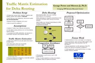
Further Improvement: Tomogravity Model (Optional Material) • Two step modeling. • Gravity Model: Initial solution obtained using edge link load data and ISP routing policy. • Tomographic Estimation: Initial solution is refined by applying quadratic programming to minimize distance to initial solution subject to tomographic constraints (link counts). CSci5221: Internet Traffic Demand and Traffic Matrix Estimation
Highlights • Router to router traffic matrix is computed instead of PoP to PoP. • Performance evaluation with real traffic matrices. • Tomogravity method (Gravity + Tomography) CSci5221: Internet Traffic Demand and Traffic Matrix Estimation
Recall: Gravity Model • General formula: • Simple gravity model: Try to estimate the amount of traffic between edge links. CSci5221: Internet Traffic Demand and Traffic Matrix Estimation
Generalized Gravity Model • Four traffic categories • Transit • Outbound • Inbound • Internal • Peers: P1, P2, … • Access links: a1, a2, ... • Peering links: p1,p2,… CSci5221: Internet Traffic Demand and Traffic Matrix Estimation
Generalized Gravity Model CSci5221: Internet Traffic Demand and Traffic Matrix Estimation
Tomography • Solution should be consistent with the link counts. CSci5221: Internet Traffic Demand and Traffic Matrix Estimation
Reducing the Computational Complexity • Hundreds of backbone routers, ten thousands of unknowns. • Observations: • Some elements of the BR to BR matrix are empty. (Multiple BRs in each PoP, shortest paths) • Topological equivalence. (Reduce the number of IGP simulations) CSci5221: Internet Traffic Demand and Traffic Matrix Estimation
Quadratic Programming • Problem Definition: • Use SVD (singular value decomposition) to solve the inverse problem. • Use Iterative Proportional Fitting (IPF) to ensure non-negativity. CSci5221: Internet Traffic Demand and Traffic Matrix Estimation
Evaluation of Gravity Models CSci5221: Internet Traffic Demand and Traffic Matrix Estimation
Performance of Proposed Algorithm CSci5221: Internet Traffic Demand and Traffic Matrix Estimation
Comparison CSci5221: Internet Traffic Demand and Traffic Matrix Estimation