Download
1 / 23
230 likes | 377 Vues
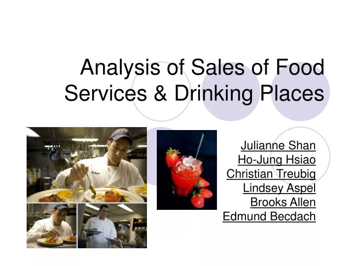
Analysis of Sales of Food Services & Drinking Places. Julianne Shan Ho-Jung Hsiao Christian Treubig Lindsey Aspel Brooks Allen Edmund Becdach. Outline. Introduction Original and Differenced data Modeling Model validation Forecasting Summary. Introduction.

E N D
Analysis of Sales of Food Services & Drinking Places Julianne Shan Ho-Jung Hsiao Christian Treubig Lindsey Aspel Brooks Allen Edmund Becdach
Outline • Introduction • Original and Differenced data • Modeling • Model validation • Forecasting • Summary
Introduction • We chose to analyze the food services and drinking industry, looking at total sales over the last 18 years or. Our data thus includes sales from many restaurants and bars across the US • As young adults, we work and spend time in these places, so we were interested to see what the trend in sales looks like
Original Data • We gathered our data from the US Census Bureau, at http://www.census.gov/marts/www/timeseries.html • The data appears to be evolutionary at first, with a clear upwards trend in sales. • Looking at the histogram of the data, we also see that the data is not Normal at the 5% significance level since the Jarque-Bera statistic has a probability of 0.00047 < 0.05; the data is slightly skewed and almost looks uniform.
Original Data • We next looked at the ACF and PACF, and found Augmented Dickey Fuller statistic of -1.54,indicating that there is a unit root at the 5% level • We found no apparent trend in the variance, but we did apply the log transformation of the data (for completeness) and there were no apparent improvements. Therefore, we chose not to apply the log transformation in our final model
Seasonal Difference • Next, we applied a seasonal difference to the data, with a seasonality of 12. The trace still looks evolutionary; there is a positive trend from 1992-2006, and a negative trend from 2006-present. • The data is now normal at the 5% level, with a Jarque-Bera statistic of probability 0.1683 > 0.05; the data is slightly skewed. • The ACF decays slowly; the PACF has significant spikes at lags 1, 2, 12, 13, 24. • The Dickey-Fuller stat shows that there is still a unit root at the 5% level
First Difference • We apply a first difference to the seasonally adjusted data, as its trace looked evolutionary; once again, the trace appears evolutionary, with a positive trend from 1992-2006, and a negative trend from 2006-present. • A look at the histogram shows that the data is not normal at the 5% significance level, since the Jarque-Bera statistic has a probability of 0.002990 < 0.05; the histogram is slightly skewed and kurtotic, but has one main peak. • The correlogram shows that the ACF has significant spikes at lags 1, 2, 11, 12, 13; the PACF has significant spikes at lags 1, 11, 12, 24, 36 • The Dickey-Fuller stat indicates that there is now NO unit root at the 5% significance level
First Difference • The correlogram shows that the ACF has significant spikes at lags 1, 2, 11, 12, 13; the PACF has significant spikes at lags 1, 11, 12, 24, 36 • The Dickey-Fuller stat indicates that there is now NO unit root at the 5% significance level
Modeling! • Since there is no unit root, the data is now stationary; we chose ten appropriate models to try to fit the data, and eventually chose the model ARIMA(1,1,1)x(1,1,1)12 • This model had the lowest AIC (Akaike Information Criterion) among the other models, at 2740 • Our last three models do not have a seasonal component, but were used to confirm that the seasonal component is necessary, as evidenced by their diagnostic plots. • The correlogram of the residuals also appears to lie within the confidence interval
Modeling! • We used the following ten models to try to estimate the trend in food service and drinking place sales: • ARIMA(1,1,1)x(0,1,0)12 • ARIMA(1,1,1)x(1,1,0)12 • ARIMA(1,1,1)x(0,1,1)12 • ARIMA(1,1,1)x(1,1,1)12 • ARIMA(0,1,2)x(1,1,1)12 • ARIMA(1,1,2)x(1,1,1)12 • ARIMA(1,1,1)x(0,0,0)12 • ARIMA(1,1,1)x(1,0,0)12 • ARIMA(1,1,1)x(0,0,1)12 • ARIMA(1,1,1)x(1,0,1)12
Modeling! • ARIMA(1,1,1)x(1,1,1)12 • AIC = 2740.571 Coefficients: ar1 ma1 -0.1516 -0.2635 s.e. 0.1813 0.1791 sar1 sma1 -0.1571 -0.9609 s.e. 0.0845 0.1794
Model Validation • From the diagnostic plots we notice the following: • The Durbin Watson Statistic = 1.98 2, indicating no serial correlation • The ACF looks like white noise: it is one at lag 1, and approximately zero at all other lags • The p-values for the Ljung-Box Statistic are all sufficiently large • The residuals are not normal since the probability of the Jarque-Bera statistic is approx. 0 < 0.05; they are slightly skewed and highly kurtotic, but there is one main peak
Model Validation • Next, we re-estimated Model 4 excluding the last 12 values (i.e. we used the data from 01/1992 – 04/2008). Then we forecasted the withheld values. • From the graph we can see that all twelve of the actual values (05/12008 – 04/2009) fall within the 95% confidence band, so our model has good predictive powers. This is our final model.
Model Validation • A plot of the actual values, forecasted values, and a 95% confidence interval:
Forecasting: • We used our final model to predict the sales of Food Services & Drinking Places (in Millions of Dollars) for the next twelve months. Our model clearly indicates that sales will continue to rise • 5/2009: $ 38,275.66 • 6/2009: $ 38,358.69 • 7/2009: $ 38,481.70 • 8/2009: $ 38,610.12 • 9/2009: $ 38,710.74 • 10/2009: $ 38,891.78 • 11/2009: $ 38,977.95 • 12/2009: $ 39,116.53 • 1/2010: $ 39,258.38 • 2/2010: $ 39,284.23 • 3/2010: $ 39,466.58 • 4/2010: $ 39,557.42
Summary • Our final model, ARIMA(1,1,1)x(1,1,1)12, predicts an increase in Food Services & Drinking Places over the next twelve months, although from the trace of the forecast it appears to be slowing down a little bit in the current recession. • This is no surprise, as our country still has a growing young population that likes to eat out and party