System Simulation Using SIMULINK: Managing Inputs, Outputs, and Dynamics
90 likes | 213 Vues
Explore the powerful functionalities of SIMULINK for simulating various systems, including both linear and nonlinear models. You can generate arbitrary input signals (e.g., sinusoidal, polynomial, step, square) and customize your simulations using functions or lookup tables. With easy parameter adjustments and initial conditions, you can visualize outputs through multiple formats. Learn step-by-step how to create models, connect components, and run simulations effectively, ensuring accurate analysis of system responses with stored results and comprehensive output demonstrations.

System Simulation Using SIMULINK: Managing Inputs, Outputs, and Dynamics
E N D
Presentation Transcript
Section 3.2.2 A Tool for System Simulation: SIMULINK • Can be used for simulation of various systems: • Linear, nonlinear; • Input signals can be arbitrarily generated: • Standard: sinusoidal, polynomial, square, impulse • Customized: from a function, look-up table • Output signals can be stored or demonstrated in • different ways.
Example: Input u Click simulation and use plot(t,y), you will get a time response of y • The parameters can be easily changed; • The initial condition can be easily changed.
The components: • Main components with dynamics: • integrators, • transfer function • zero-pole description • The first one needs an initial condition. • It can be assigned by clicking on the • component • Math components: • gain (amplifier) kx : x a scalar • addition (a+b+c); product (ab); you can change the number of terms and the sign of each term
Sources: input signals • constant, step, ramp • pulse, sine wave, square wave • from data file • signal generator • The clock to record time • Sinks: for output demonstration or storage • export to workspace; you can give a name to the variable, such as u, y, x, etc. • scope • digital display
Example: Find the solution to the systems where y(0)=0; y’(0)=0. u(t) is a square wave. • Steps: • Open matlab workspace • type simulink and return • - simulink library browser window is open • Click file and choose new then choose model • - a blank window is open • Open one of the commonly used blocks and drag and drop • whatever you need to the blank window. • 5. Connect the components by arrows.
Click each component to setup the parameters properly • sinks labeled “t”, “u”, “y”: choose “array” for save format • sampling time can be a parameter inputted from workspace • they can be chosen as -1 for inherited • When ready, click simulation and choose configuration parameters • to setup simulation time. Finally, click simulation and choose start • When finished, type plot(t,y,t,u) to plot the input and output
How to realize and then realize Can we first get Theoretically, we need future information of u(t), t > t0 to get the derivative at t0. This cannot be realized. We may only use the past information to get an approximation. But still it is better not to use differentiator. If a signal is contaminated by noises, taking derivative will magnify the noises. One approach to avoid differentiation is as follows: - First realize Initial condition determined from Then set -You can verify that y satisfies (*).
- -