Download
1 / 39
400 likes | 533 Vues
Seismology Part III: Body Waves and Ray Theory in Layered Medium. Rays in layered medium are simple, and also very useful in a lot of applications. Rays within layers are straight lines (wavespeed is constant).

E N D
Seismology Part III: Body Waves and Ray Theory in Layered Medium
Rays in layered medium are simple, and also very useful in a lot of applications. Rays within layers are straight lines (wavespeed is constant). Rays at boundaries refract according to Snell’s law (or, in other words, they keep the same ray parameter). Travel time is the length of the straight line path divided by the wavespeed. There are three types of path to consider: 1. Direct/transmitted/refracted 2. Critically refracted (head) 3. Reflected
Suppose we have an interface separating two media with wavespeeds c1 and c2. Consider a wave in c1 approaching an interface at an angle i w.r.t. the normal to the interface. The transmitted wave leaves with the angle it, and the reflected wave with the angle ir. Then And so
it cannot be greater than 90o for a transmitted wave. We define the critical angle as: Note that ic can exist only if c2 > c1. When this happens, a (head) wave is transmitted along the interface, traveling at a speed of c2.
For a single layer over a half space, simple geometry gives: Note that for a head wave
Substituting in for the expression for head wave time: where Note that T is proportional to X (minus a constant). Where did we see that before?
In multiple layers, we can write this as: It is generally useful to plot seismograms in an X vs T plot to identify coherent arrivals. We interpret these arrivals by comparing with theory. For a layer over a half space, the direct and head waves are straight lines on an X-T plot, and the reflected wave is a hyperbola that asymptotically approaches the head wave.
Note that for the reflected wave So a plot of T2 vs X2 gives a straight line, and T vs X is a hyperbola. There is no exact extension to multiple layers, but approximate formulas are often used.
The refracted arrival will overtake the direct arrival when This crossover distance is useful to know when planning a refraction experiment (i.e., how far away must sensors be in order to detect a refracted first motion?).
Some headaches of refraction seismology: • 1. Low velocity layers: these cannot be detected and will give false depths to interfaces. Nothing can be done about this.
2. Blind zones: Thin layers; too thin for the refracted arrival to ever arrive first. Can sometimes see in the background, but usually ambiguous.
3. Dipping Layers: Look just like flat layers but will give wrong wavespeed and thickness. Remedy is to “reverse” the profile. Here is how you do it:
Downdip travel time can be shown with simple trig to be: Updip travel time is where hd and hu are the downdip and updip depths to the layers, and is the dip. Note that both of these X-T equations are straight lines with different slopes and intercepts. This asymmetry is diagnostic of a dipping interface, and this is why we always “reverse” the refraction profile.
Note that we can determine the dip, depth, and wavespeeds of the medium by: and the depth can be determined from the intercepts:
ALTERNATE REALITIES A useful way to summarize travel time data is as a -p plot, where p will be the slope (=1/c) and will be the intercept. X-T, X-p, and -p plots all have the same information in the, its just that this information can be more readily understood in some frames.
Spherical Earth The ideas above developed for a flat earth are easily extended to a spherical earth. Imagine a spherical interface. At the interface, Snell holds: Now extend the ray to a deeper interface. From the diagram, d is the common distance along a right triangle formed by the ray extension, and
This will be true as the width becomes infinitesimally small. So, in general Also, near the surface, simple geometry shows: Remember that "" is in radians!
Travel Time and Distance in a Sphere Consider a spherical ray segment: and so and
Solve for d: Integrate the above from ro to rmin (maximum depth of penetration) and multiply by 2 to get total distance:
We follow similar steps to get travel time by integrating solving for ds instead of d and then integrating ds/c: Note that this can be written like a -p equation like in flat earth by combining the above with the expression for :
What happens at an interface: • Energy partitioning at a boundary. • We would like to know what happens when a propagating displacement encounters a boundary, and specifically how does the displacement on one side influence that on the other side. To do so, we need to consider what happens with displacements and tractions on the boundary. • First, what kinds of boundaries do we have to deal with? • Solid-Solid or Welded interface. All points move together. • Solid-Liquid (and Liquid-Liquid). Vertical motion continuous • Free Surface. No constraint on displacement
Solid-Solid or Welded interface. All points move together. In this case Displacement and Traction are continuous across the boundary. Displacement is easy to visualize, here is why traction is: Imagine a volume V surrounding the interface; V=Adz. From the homogeneous equation of motion (no sources in V), we have: From the divergence theorem:
So where n is normal to the surfaces parallel to the interface. Now, as dz goes to zero, dV goes to zero faster than dS, so it must be that which means that the Tractions on either side must be equal (i.e., continuous).
2. Solid-Liquid (and liquid-liquid). Normal components of displacement and traction are continuous. Shear displacement is unconstrained. Shear traction is zero. 3. Free Surface. No displacement constraint. Traction is zero. (That’s why it’s free!)
Suppose we have two layers, 1 and 2, separated by an interface. Let's consider the case of a P wave incident in layer 1 upon the interface. The potentials in layer 1 will be the sum of incident and reflected P and the potential due to a reflected SV wave: The potentials in layer 2 will be the refracted P and SV waves:
We can write the solution to the wave equations as: The signs in the arguments that correspond to the direction of propagation, and the appropriate choices of the x3 factors. Also, the x1 factor is the same in every case because of Snell's law. Now
So, in general, we consider the displacements at the interface substituting the above expressions into the following: The continuity of u across the interface means uxi+ = uxi- (as appropriate). For the traction condition, we convert traction to stress using and then go from stress to strain using the linear elastic constitutive equation, and finally to displacement by taking spatial derivatives.
Note that if the interface is horizontal, then n = (0,0,1) and The “answer” is to determine the relation between the incident and reflected/refracted energy. For the most part this is simply a question of algebra. Let’s look at a simple case of P waves at a liquid-liquid interface ( = 0 so no S waves) in the x1-x3 plane (i.e., no displacements in the x2 direction). In this case the displacement field is
At a liquid-liquid interface, only the vertical component is continuous, so Thus or, for convenience we choose x3 = 0, then
Continuity of traction. In a liquid/liquid case, only the normal component is continuous: and from our constitutive equation: because = 0 in a liquid. The scalar potential
Thus So Sum the above
Eliminating A3 from the above: or Now, note that these relationships are for the amplitudes of the scalar potential function, not of the displacement. To recover displacement, recall that
Note that at normal incidence, p = 0, so 1= 1/1, 2= 1/2 and so in this case
The product is called the seismic impedance. Note that it is the impedance contrast that is most important in determining how much energy is reflected. There is a simple general relationship between the reflection and transmission coefficients that holds for any interface and for any angle: T = 1+R R can vary between –1 and 1, which means that T goes between 0 and 2. R = 1 at a free surface, which means that we generally will record a wave at twice its normal amplitude. These expressions allow us to understand quantitatively what happens at an interface when the angle of incidence is greater than or equal to the critical angle.
Recall that when i = ic, n2 = 0. When i1 > ic, n2 is imaginary: This means that the transmitted wave will decay exponentially with distance away from the interface. The reflection coefficient becomes:
This is just a complex number divided by its complex conjugate. We know immediately then than the magnitude of R is 1, and that there will be a phase shift in the amount: So, beyond the critical angle, we have total internal reflection (R = 1) and there will be some distortion because of the phase shift. To quantify this distortion, note that we can write the potential of the postcritical reflection as: which means that the phase of the wave (constant argument) is a function of frequency.
The term can be thought of as an apparent time. Since < 0, lower frequencies will have earlier arrival times than higher frequencies, which means the wave is dispersed (spread out). The transmission coefficient is Note that in general, an incident P wave will generate (Prefl, Srefl, Ptrans, Strans) so we get 4 waves generated for every one incident. Same with SV. SH produces only an SH wave.