Linear scaling solvers based on Wannier-like functions
310 likes | 453 Vues
This paper presents linear scaling solvers derived from Wannier-like functions to achieve efficient density functional theory (DFT) computations. The focus is on methodologies that permit an Order(N) scaling in computational load for large systems, allowing for the treatment of up to 132,000 atoms with reduced resource demands. Key insights include locality principles and minimization techniques to optimize wave functions and energy functional calculations. Additionally, it discusses practical implementations, convergence challenges, and the advantages of using localized wave functions in DFT frameworks.

Linear scaling solvers based on Wannier-like functions
E N D
Presentation Transcript
Linear scaling solvers based on Wannier-like functions P. Ordejón Institut de Ciència de Materials de Barcelona (CSIC)
Linear scaling = Order(N) CPU load 3 ~ N ~ N Early 90’s ~ 100 N (# atoms)
Order-N DFT • Find density and hamiltonian (80% of code) • Find “eigenvectors” and energy (20% of code) • Iterate SCF loop • Steps 1 and 3 spared in tight-binding schemes
Key to O(N): locality Large system ``Divide and conquer’’W. Yang, Phys. Rev. Lett. 66, 1438 (1992) ``Nearsightedness’’W. Kohn, Phys. Rev. Lett. 76, 3168 (1996)
1 = 1/2 (Ψ1+Ψ2) Ψ2 Ψ1 2 = 1/2 (Ψ1-Ψ2) Locality of Wave Functions Wannier functions (crystals) Localized Molecular Orbitals (molecules)
Locality of Wave Functions Energy: Unitary Transformation: We do NOT need eigenstates! We can compute energy with Loc. Wavefuncs.
610-21 7.6 Locality of Wave Functions Exponential localization (insulators): Wannier function in Carbon (diamond) Drabold et al.
Locality of Wave Functions Insulators vs Metals: Carbon (diamond) Aluminium Goedecker & Teter, PRB 51, 9455 (1995)
Linear Scaling Localization + Truncation • Sparse Matrices 5 4 • Truncation errors 2 1 3 In systems with a gap. Decay rate a depends on gap Eg
Linear Scaling Approaches • (Localized) object which is computed: • - wave functions • - density matrix • Approach to obtain the solution: • - minimization • - projection • spectral • Reviews on O(N) Methods: Goedecker, RMP ’98 • Ordejón, Comp. Mat. Sci.’98
Basis sets for linear-scaling DFT • LCAO: - Gaussian based + QC machinery • M. Challacombe, G. Scuseria, M. Head-Gordon ... • - Numerical atomic orbitals (NAO) • SIESTA • S. Kenny &. A Horsfield (PLATO) • OpenMX • Hybrid PW – Localized orbitals • - Gaussians J. Hutter, M. Parrinello • - “Localized PWs” • C. Skylaris, P, Haynes & M. Payne • B-splines in 3D grid • D. Bowler & M. Gillan • Finite-differences (nearly O(N)) • J. Bernholc
x central b c b buffer buffer central buffer x’ Divide and conquer Weitao Yang (1992)
1 0 Emin EF Emax Fermi operator/projector Goedecker & Colombo (1994) f(E) = 1/(1+eE/kT) n cn En F cn Hn Etot = Tr[ F H ] Ntot = Tr[ F ] ^ ^ ^ ^ ^
= 3 2 - 2 3 Etot() = H = min 1 0 -0.5 0 1 1.5 Density matrix functional Li, Nunes & Vanderbilt (1993)
Sij = < i | j > | ’k > = j | j > Sjk-1/2 EKS = k< ’k | H | ’k > = ijk Ski-1/2< i | H | j > Sjk-1/2 = Trocc[ S-1 H ] Kohn-Sham EOM = Trocc[ (2I-S) H ] Order-N = Trocc[ H] + Trocc[(I-S) H ] ^ ^ Wannier O(N) functional • Mauri, Galli & Car, PRB 47, 9973 (1993) • Ordejón et al, PRB 48, 14646 (1993)
O(N) Non-orthogonality penalty KS Sij = ij EOM = EKS Order-N vs KS functionals
Chemical potential Kim, Mauri & Galli, PRB 52, 1640 (1995) • (r) = 2ij i(r) (2ij-Sij) j(r) • EOM = Trocc[ (2I-S) H ]# states = # electron pairs • Local minima • EKMG = Trocc+[ (2I-S) (H-S) ]# states > # electron pairs = chemical potential (Fermi energy) Ei > |i| 0 Ei < |i| 1 Difficulties Solutions • Stability of N() Initial diagonalization / Estimate of • First minimization of EKMG Reuse previous solutions
i Rc rc Orbital localization i(r) = ci(r)
Convergence with localisation radius Si supercell, 512 atoms Relative Error (%) Rc (Ang)
x i x 0 2 5.37 5.37 3 1.85 8.29 1.85 = 15.34 3.14 0 = 0 1.15 0 = 0 ------- Sum 15.34 1.85 7 2.12 0 0 i y 0 2.12 3 8.29 0 4 3.14 8 1.15 Sparse vectors and matrices Restore to zero xi 0 only
Actual linear scaling c-Si supercells, single- Single Pentium III 800 MHz. 1 Gb RAM 132.000 atoms in 64 nodes
Linear scaling solver: practicalities in SIESTA P. Ordejón Institut de Ciència de Materials de Barcelona (CSIC)
Order-N in SIESTA (1) Calculate Hamiltonian Minimize EKS with respect to WFs (GC minimization) Build new charge density from WFs SCF
Energy Functional Minimization • Start from initial LWFs (from scratch or from previous step) • Minimize Energy Functional w.r.t. ci • EOM = Trocc[ (2I-S) H ] or • EKMG = Trocc+[ (2I-S) (H-S) ] • Obtain new density • (r) = 2ij i(r) (2ij-Sij) j(r) ci(r) = ci(r)
i Rc rc Orbital localization i(r) = ci(r)
Order-N in SIESTA (2) • Practical problems: • Minimization of E versus WFs: • First minimization is hard!!! (~1000 CG iterations) • Next minimizations are much faster (next SCF and MD steps) • ALWAYS save SystemName.LWF and SystemName.DM files!!!! • The Chemical Potential (in Kim’s functional): • Data on input (ON.Eta). Problem: can change during SCF and dynamics. • Possibility to estimate the chemical potential in O(N) operations • If chosen ON.Eta is inside a band (conduction or valence), the minimization often becomes unstable and diverges • Solution I: use chemical potential estimated on the run • Solution II: do a previous diagonalization
Example of instability related to a wrong chemical potential
Order-N in SIESTA (3) • SolutionMethod OrderN • ON.Functional Ordejon-Mauri or Kim (def) • ON.MaxNumIter Max. iterations in CG minim. (WFs) • ON.Etol Tolerance in the energy minimization 2(En-En-1)/(En+En-1) < ON.Etol • ON.RcLWF Localisation radius of WFs
Order-N in SIESTA (4) • ON.Eta (energy units) Chemical Potential (Kim) Shift of Hamiltonian (Ordejon-Mauri) • ON.ChemicalPotential • ON.ChemicalPotentialUse • ON.ChemicalPotentialRc • ON.ChemicalPotentialTemperature • ON.ChemicalPotentialOrder
1 0 Emin EF Emax Fermi operator/projector Goedecker & Colombo (1994) f(E) = 1/(1+eE/kT) n cn En F cn Hn Etot = Tr[ F H ] Ntot = Tr[ F ] ^ ^ ^ ^ ^