Download
1 / 25
290 likes | 366 Vues
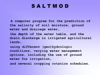
SALTMOD is a computer program for predicting soil moisture salinity, water table depth, and drainage discharge in irrigated lands. It aids in managing water resources efficiently, incorporating crop rotations and irrigation practices.

E N D
A computer program for the prediction of the salinity of soil moisture, ground water and drainage water, the depth of the water table, and the drain discharge in irrigated agricultural lands, using different (geo)hydrologic conditions, varying water management options, including the use of ground water for irrigation, and several cropping rotation schedules. S A L T M O D
Design requirements of Saltmod • The model should be simple and it should not require a PhD degree to operate it. • The input data should be readily available or relatively easy to obtain. • The model should be able to integrate agricultural, irrigation and drainage practices. • The results can be checked by hand. • The data can be imported into spreadsheet (e.g. Excel) for further analysis.
In the soil profile we recognise 4 reservoirs: • 1 On top of soil surface • 2 Root zone/Evapotranspiration zone • 3 Transition zone • 4 Aquifer • Salt and water balances are made for each reservoir: • Inflow = outflow + change in storage
Seasons • Maximum 4 agricultural seasons • Maximum 3 types of land use per season • (A, B, U) to be defined by user. • Example Garmsar, 3 seasons • Nov-Apr A=wheat+barley 30% • B=0, U=70% (no irrigation) • May-Aug A=cotton (20%) B=melon (10%) • U=70% (no irrigation) • Sept-Oct A=0, B=0, U=100%
Crop rotations • Together with previous cropping data, the crop rotations must be specified. • Rotation code Kr = 0, 1, 2, 3, 4 0 = no crop rotation (fixed areas e.g. Sugarcane, orchards) 4 = full rotation (no fixed areas) 1 = fallow area is fixed, permanent, other crops have full rotation • Etcetera • In Garmsar use Kr=4
The irrigation water can incorporate re-use of groundwater and drainage water
The complex capillary rise function is simplified and only critical depth Dc of water table is used, depending on soil type
Characteristics of drainage systems are introduced in a simple way using well known drain spacing equations. For details see manual.
Example of partition of fallow land (U) into permanent fallow (Uc) and temporary fallow (U-Uc) when Kr = 1.Pooling of percolation/leaching (L) and capillary rise (R) in the part of the area that is under full rotation
The salinity of the topsoil decreases rapidly (good leaching).Salinity of transition zone first increases slightly, then decreases.Salinity of the aquifer shows slow reaction.
Saltmod calculates average salinity and an empirical frequency distribution is used to characterise spatial variation
Case study Egypt Saltmod was used in Egypt see if drainage systems could be made less expensive. However, the leaching efficiency of salts was not known. It had to be found by trials with the model (calibration). Various leaching efficiencies were tried: 20%, 40%, 60%, 80% etc. The salinity results were compared to actually measured results and the true efficiency could be found (next slide).
Conclusion • The leaching efficiency (FLr) is definitely greater than 0.6, because smaller values give results that deviate too much from the observed values. • Flr is definitely smaller than 1 for the same reason. • The true Flr is about 0.8 • A small error of Flr in the range between 0.7 and 0.8 does not have too much influence on soil salinity, so OK.
Calibrating groundwater flow • As the groundwater flow was unknown it had to be found by calibration • Previous reports indicated that no upward seepage occurs but rather some natural drainage through the underground • Therefore trials were made with annual values of natural drainage Gn = 0.0, 0.07, 0.14, 0.21 and 0.28 m • The results are shown in the next table.
Observed values: • Depth of water table: Dw 1st season (summer) 1.0 – 1.1 m Dw 2nd season (winter) 1.2 – 1.3 m • Drain discharge: Gd 1st season 100 – 150 mm Gd 2nd season 50 – 100 mm • Compare with previous slide and conclude that the natural drainage (Gn) to the underground should be between 0.70 and 0.21 m/year.
Conclusion • The value of natural drainage Gn cannot be determined with great precision due to variation of data, but it cannot be less than 0.07 and more than 0.21 m/year • We will accept the average Gn=0.14 as the true value. • Herewith Gn is determined by the model and the model is calibrated.
Simulating drain depth Question: Is it justified to use in practice drain depths of 1.0 m instead of standard practice 1.4 m so that savings can be made on installation costs ?
Field measurements showed that most crops have no yield reduction when the depth of water table is 0.6 m. Why make it deeper?
Conclusion The previous table shows that with drain depth = 1.0 m: • the depth of the water table is OK • the soil salinity is slightly higher, but OK • the irrigation efficiency is slightly better • the irrigation sufficiency is slightly better