Download
1 / 48
490 likes | 536 Vues
Dive into the principles of thermofluid mechanics with Navier-Stokes equations and computational fluid dynamics. Explore conservation laws, control volume analysis, and velocity derivatives crucial for fluid motion analysis.

E N D
ME 231 Thermofluid Mechanics I Navier-Stokes Equations
Computational Fluid Dynamics (AE/ME 339) K. M. Isaac MAEEM Dept., UMR • Equations of Fluid Dynamics, Physical Meaning of the terms. • Equations are based on the following physical principles: • Mass is conserved • Newton’s Second Law: • The First Law of thermodynamics: De = dq - dw, for a system.
Computational Fluid Dynamics (AE/ME 339) K. M. Isaac MAEEM Dept., UMR Control Volume Analysis The governing equations can be obtained in the integral form by choosing a control volume (CV) in the flow field and applying the principles of the conservation of mass, momentum and energy to the CV.
Computational Fluid Dynamics (AE/ME 339) K. M. Isaac MAEEM Dept., UMR
Computational Fluid Dynamics (AE/ME 339) K. M. Isaac MAEEM Dept., UMR • Consider a differential volume element dV in the flow field. dV is small enough to be considered infinitesimal but large enough to contain a large number of molecules for continuum approach to be valid. • dV may be: • fixed in space with fluid flowing in and out of its surface or, • moving so as to contain the same fluid particles all the time. In this case the boundaries may distort and the volume may change.
Computational Fluid Dynamics (AE/ME 339) K. M. Isaac MAEEM Dept., UMR Substantial derivative (time rate of change following a moving fluid element)
Computational Fluid Dynamics (AE/ME 339) K. M. Isaac MAEEM Dept., UMR The velocity vector can be written in terms of its Cartesian components as: where u = u(t, x, y, z) v = v(t, x, y, z) w = w(t, x, y, z)
Computational Fluid Dynamics (AE/ME 339) K. M. Isaac MAEEM Dept., UMR @ time t1: @ time t2: Using Taylor series
Computational Fluid Dynamics (AE/ME 339) K. M. Isaac MAEEM Dept., UMR The time derivative can be written as shown on the RHS in the following equation. This way of writing helps explain the meaning of total derivative.
Computational Fluid Dynamics (AE/ME 339) K. M. Isaac MAEEM Dept., UMR We can also write
Computational Fluid Dynamics (AE/ME 339) K. M. Isaac MAEEM Dept., UMR where the operator can now be seen to be defined in the following manner.
Computational Fluid Dynamics (AE/ME 339) K. M. Isaac MAEEM Dept., UMR The operator in vector calculus is defined as which can be used to write the total derivative as
Computational Fluid Dynamics (AE/ME 339) K. M. Isaac MAEEM Dept., UMR Example: derivative of temperature, T
Computational Fluid Dynamics (AE/ME 339) K. M. Isaac MAEEM Dept., UMR A simpler way of writing the total derivative is as follows:
Computational Fluid Dynamics (AE/ME 339) K. M. Isaac MAEEM Dept., UMR The above equation shows that and have the same meaning, and the latter form is used simply to emphasize the physical meaning that it consists of the local derivative and the convective derivatives. Divergence of Velocity (What does it mean?) Consider a control volume moving with the fluid. Its mass is fixed with respect to time. Its volume and surface change with time as it moves from one location to another.
Computational Fluid Dynamics (AE/ME 339) K. M. Isaac MAEEM Dept., UMR Insert Figure 2.4
Computational Fluid Dynamics (AE/ME 339) K. M. Isaac MAEEM Dept., UMR The volume swept by the elemental area dS during time interval Dt can be written as Note that, depending on the orientation of the surface element, Dv could be positive or negative. Dividing by Dt and letting 0 gives the following expression.
Computational Fluid Dynamics (AE/ME 339) K. M. Isaac MAEEM Dept., UMR The LHS term is written as a total time derivative because the fluid element is moving with the flow and it would undergo both the local acceleration and the convective acceleration. The divergence theorem from vector calculus can now be used to transform the surface integral into a volume integral.
Computational Fluid Dynamics (AE/ME 339) K. M. Isaac MAEEM Dept., UMR If we now shrink the moving control volume to an infinitesimal volume, , , the above equation becomes When the volume integral can be replaced by on the RHS to get the following. The divergence of is the rate of change of volume per unit volume.
Computational Fluid Dynamics (AE/ME 339) K. M. Isaac MAEEM Dept., UMR
Computational Fluid Dynamics (AE/ME 339) K. M. Isaac MAEEM Dept., UMR Continuity Equation Consider the CV fixed in space. Unlike the earlier case the shape and size of the CV are the same at all times. The conservation of mass can be stated as: Net rate of outflow of mass from CV through surface S = time rate of decrease of mass inside the CV
Computational Fluid Dynamics (AE/ME 339) K. M. Isaac MAEEM Dept., UMR The net outflow of mass from the CV can be written as Note that by convention is always pointing outward. Therefore can be (+) or (-) depending on the directions of the velocity and the surface element.
Computational Fluid Dynamics (AE/ME 339) K. M. Isaac MAEEM Dept., UMR Total mass inside CV Time rate of increase of mass inside CV (correct this equation) Conservation of mass can now be used to write the following equation See text for other ways of obtaining the same equation.
Computational Fluid Dynamics (AE/ME 339) K. M. Isaac MAEEM Dept., UMR Integral form of the conservation of mass equation thus becomes
Computational Fluid Dynamics (AE/ME 339) K. M. Isaac MAEEM Dept., UMR
Computational Fluid Dynamics (AE/ME 339) K. M. Isaac MAEEM Dept., UMR An infinitesimally small element fixed in space
Computational Fluid Dynamics (AE/ME 339) K. M. Isaac MAEEM Dept., UMR Net outflow in x-direction Net outflow in y-direction Net outflow in z-direction Net mass flow =
Computational Fluid Dynamics (AE/ME 339) K. M. Isaac MAEEM Dept., UMR volume of the element = dx dy dz mass of the element = r(dx dy dz) Time rate of mass increase = Net rate of outflow from CV = time rate of decrease of mass within CV or
Computational Fluid Dynamics (AE/ME 339) K. M. Isaac MAEEM Dept., UMR Which becomes The above is the continuity equation valid for unsteady flow Note that for steady flow and unsteady incompressible flow the first term is zero. Figure 2.6 (next slide) shows conservation and non-conservation forms of the continuity equation. Note an error in Figure 2.6: Dp/Dt should be replace with Dr/Dt.
Computational Fluid Dynamics (AE/ME 339) K. M. Isaac MAEEM Dept., UMR
Computational Fluid Dynamics (AE/ME 339) K. M. Isaac MAEEM Dept., UMR Momentum equation
Computational Fluid Dynamics (AE/ME 339) K. M. Isaac MAEEM Dept., UMR Consider the moving fluid element model shown in Figure 2.2b Basis is Newton’s 2nd Law which says F = m a Note that this is a vector equation. It can be written in terms of the three cartesian scalar components, the first of which becomes Fx = m ax Since we are considering a fluid element moving with the fluid, its mass, m, is fixed. The momentum equation will be obtained by writing expressions for the externally applied force, Fx, on the fluid element and the acceleration, ax, of the fluid element. The externally applied forces can be divided into two types:
Computational Fluid Dynamics (AE/ME 339) K. M. Isaac MAEEM Dept., UMR • Body forces: Distributed throughout the control volume. Therefore, • this is proportional to the volume. Examples: gravitational forces, • magnetic forces, electrostatic forces. • Surface forces: Distributed at the control volume surface. Proportional • to the surface area. Examples: forces due to surface and normal stresses. • These can be calculated from stress-strain rate relations. • Body force on the fluid element = fxr dx dy dz • where fx is the body force per unit mass in the x-direction • The shear and normal stresses arise from the deformation of the fluid • element as it flows along. The shape as well as the volume of the fluid • element could change and the associated normal and tangential stresses • give rise to the surface stresses.
Computational Fluid Dynamics (AE/ME 339) K. M. Isaac MAEEM Dept., UMR
Computational Fluid Dynamics (AE/ME 339) K. M. Isaac MAEEM Dept., UMR The relation between stress and rate of strain in a fluid is known from the type of fluid we are dealing with. Most of our discussion will relate to Newtonian fluids for which Stress is proportional to the rate of strain For non-Newtonian fluids more complex relationships should be used. Notation: stress tij indicates stress acting on a plane perpendicular to the i-direction (x-axis) and the stress acts in the direction, j, (y-axis). The stresses on the various faces of the fluid element can written as shown in Figure 2.8. Note the use of Taylor series to write the stress components.
Computational Fluid Dynamics (AE/ME 339) K. M. Isaac MAEEM Dept., UMR The normal stresses also has the pressure term. Net surface force acting in x direction =
Computational Fluid Dynamics (AE/ME 339) K. M. Isaac MAEEM Dept., UMR
Computational Fluid Dynamics (AE/ME 339) K. M. Isaac MAEEM Dept., UMR
Computational Fluid Dynamics (AE/ME 339) K. M. Isaac MAEEM Dept., UMR
Computational Fluid Dynamics (AE/ME 339) K. M. Isaac MAEEM Dept., UMR The term in the brackets is zero (continuity equation) The above equation simplifies to Substitute Eq. (2.55) into Eq. (2.50a) shows how the following equations can be obtained.
Computational Fluid Dynamics (AE/ME 339) K. M. Isaac MAEEM Dept., UMR The above are the Navier-Stokes equations in “conservation form.”
Computational Fluid Dynamics (AE/ME 339) K. M. Isaac MAEEM Dept., UMR For Newtonian fluids the stresses can be expressed as follows
Computational Fluid Dynamics (AE/ME 339) K. M. Isaac MAEEM Dept., UMR • In the above m is the coefficient of dynamic viscosity and l is the second • viscosity coefficient. • Stokes hypothesis given below can be used to relate the above two • coefficients • l = - 2/3 m • The above can be used to get the Navier-Stokes equations in the following • familiar form
Computational Fluid Dynamics (AE/ME 339) K. M. Isaac MAEEM Dept., UMR
Computational Fluid Dynamics (AE/ME 339) K. M. Isaac MAEEM Dept., UMR The energy equation can also be derived in a similar manner.
Computational Fluid Dynamics (AE/ME 339) K. M. Isaac MAEEM Dept., UMR The above equations can be simplified for inviscid flows by dropping the terms involving viscosity.
Summary • Apply conservation equations to a control volume (CV) • As the CV shrinks to infinitesimal volume, the resulting partial • differential equations are the Navier-Stokes equations • Taylor series can be used to write the variables • The total derivative consists of local time derivative and convective • derivative terms • In incompressible flow, divergence of velocity is a statement of • the conservation of volume • Need surface and body forces to write the momentum equation • Surface forces are: pressure forces, forces due to normal stresses • and forces due to shear stresses • Body forces are due to weight, magnetism and electrostatics • Momentum equation is a vector equation. Can be written in terms • of its components.
Summary • Stresses are indicated by a plane and a direction, respectively, by two subscripts • For Newtonian fluids, stresses are proportional to the rates of strain • Stokes hypothesis is used to relate the first and second coefficients of viscosity • The resulting equations are the Navier-Stokes equations • In order to solve the equations, they must be simplified for the problem • you are considering (e. g., boundary layer, jet, airfoil flow, nozzle flow)