Multiple-key indexes
240 likes | 395 Vues
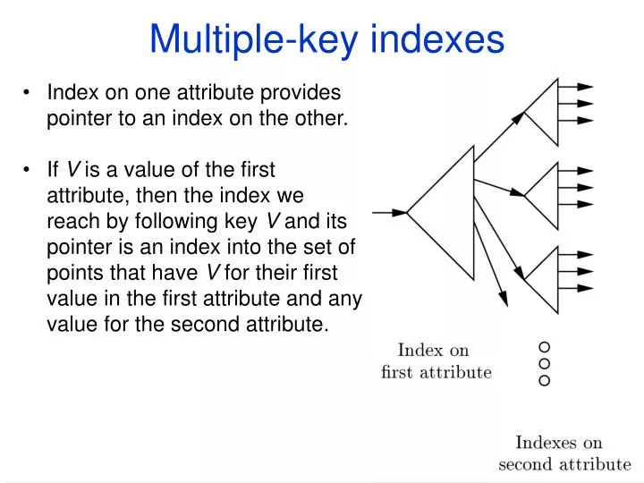
Multiple-key indexes. Index on one attribute provides pointer to an index on the other.

Multiple-key indexes
E N D
Presentation Transcript
Multiple-key indexes • Index on one attribute provides pointer to an index on the other. • If V is a value of the first attribute, then the index we reach by following key V and its pointer is an index into the set of points that have V for their first value in the first attribute and any value for the second attribute.
Example • ``Who buys gold jewelry'' (age and salary only). Raw data in agesalary pairs: (25; 60) (45; 60) (50; 75) (50; 100) (50; 120) (70; 110) (85; 140) (30; 260) (25; 400) (45; 350) (50; 275) (60; 260) • Question: For what kinds of queries will a multiplekey index (age first) significantly reduce the number of disk I/O's? The indexes can be organized as B-Trees.
Operations Partial match queries • If the first attribute is specified, then the access is quite efficient • If the first attribute isn’t specified, then we have to search every sub-index. Range queries • Quite well, provided the individual indexes themselves support range queries on their attribute (e.g. they are B-Trees) • Example. Range query is 35age55 AND 100sal200 NN queries • Similar to range queries. Also, the sub-indexes should be “primary” ones if we want to support efficiently range queries.
KD-Trees • Generalizes binary search trees, but search attributes rotate among dimensions • Levels rotate among the dimensions, partitioning the points by comparison with a value for that dimension. • Leaves are blocks
Geometrically… • Remember we didn’t want the stripes in grid files to continue all along the vertical or horizontal direction? • Here they don’t.
Operations Lookup in KDTrees • Find appropriate leaf by binary search. Is the record there? Insert Into KDTrees • Lookup record to be inserted, reaching the appropriate leaf. • If there is room, put record in that block. • If not, find a suitable value for the appropriate dimension and split the leaf block. Example • Someone 35 years old with a salary of $500K buys gold jewelry. • Belongs in leaf with (25; 400) and (45; 350). • Too full: split on age. See figure next.
Queries Partial match queries • When we don’t know the value of the attribute at the node, we must explore both of its children. • E.g. find points with age=50 Range Queries • Sometimes a range will allow us to move to only one child of a node. • But if the range straddles the splitting value then we must explore both children.
KD-trees in secondary storage • 1000 leaves log2(1000) = 10 levels. • If each internal node is stored in one block then too many disk I/O’s • Solution: Group nodes into blocks
400 Sal g b h d e a k c f j l i Age 50, Sal 200 0 Age 100 i h c e Age 75, Sal 100 Age 25, Sal 300 a b f g l j k d Quad trees • Nodes split at all dimensions at once • For a quad tree of k dimension, each interior node has 2k children. • Division fixed; tree can’t be balanced
Why quad trees? • k-dimensions node has 2k children, e.g. k=7 128 children. • We can pack all children of a node in 1 block
QuadTree Insert and Queries Insert • Find leaf node in which new point belongs. • If room, put it there. • If not, make the leaf an interior node and give it leaves for each quadrant. Split the points among the new leaves. • Problem: may make lots of null pointers, especially in highdimensions. QuadTree Queries • Single point queries: easy; just go down the tree to proper leaf. • Range queries: varies by position of range. • Example: a range like 45<age<55; 180<salary<220 requires search of four leaves, none of which is guaranteed to produce any answers. • But if range covers a large subtree of the quad tree, then even if we have to search a large number of leaves, we know that everything we find is an answer. Nearest neighbor: Problems and strategies similar to grid files.
R-Trees • For “regions” (typically rectangles) but can represent points. • Supports NN, “whereamI” queries. • Generalizes Btree to multidimensional case. • Problem: no ideal way to partition children without overlap. • In place of Btree's keypointer pairs, Rtree has regionpointer pairs.
Lookup • We start at the root, with which the entire region is associated. • We examine the subregions at the root and determine which children correspond to interior regions that contain point P. • If there are zero regions we are done; P is not in any data region. • If there are some subregions we must recursively search those children as well, until we reach the leaves of the tree.
Insertion • We start at the root and try to find some subregion into R fits. If more than one we pick just one, and repeat the process there. • If there is no region, we expand, and we want to expand as little as possible. So, we pick the child that will be expanded as little as possible. • Eventually we reach a leaf, where we insert the region R. • However, if there is no room we have to split the leaf. We split the leaf in such a way as to have the smallest subregions.
Example • Suppose that the leaves have room for six regions. • Further suppose that the six regions are together on one leaf, whose region is represented by the outer solid rectangle. • Now suppose that another region POP is added.
Example (Cont’ ed) ((0,0),(60,50)) ((20,20),(100,80)) Road1 Road2 House1 School House2 Pipeline Pop
Example (Cont’ ed) • Suppose now that House3 ((70,5),(80,15)) gets added. • We do have space to the leaves, but we need to expand one of the regions at the parent. • We choose to expand the one which needs to be expanded the least.
Which one should we expand? ((0,0),(80,50)) ((20,20),(100,80)) Road1 Road2 House1 House3 School House2 Pipeline Pop ((0,0),(60,50)) ((5,20),(100,80)) Road1 Road2 House1 School House2 Pipeline Pop House3
Bitmap Indexes • Suppose we have n tuples. • A bitmap index for a field F is a collection of bit vectors of length n, one for each possible value that may appear in the field F. • The vector for value v has 1 in position i if the i-th record has v in field F, and it has 0 there if not. (30, foo) (30, bar) (40, baz) (50, foo) (40, bar) (30, baz) foo 100100 bar 0… baz …
Motivation for Bitmap Indexes • They allow very fast evaluation of partial match queries. SELECT title FROM Movie WHERE studioName=‘Disney’ AND year=1995; If there are bitmap indexes on both studioName and year, we can intersect the vectors for the Disney value and 1995 value. We should have another index to retrieve the tuples by number.
Compressed Bitmaps 00000000000001 i-1 in unary and followed by the binary representation. i=4 Encoding: 1110