Douglas-fir mortality estimation with generalized linear mixed models
280 likes | 470 Vues
Douglas-fir mortality estimation with generalized linear mixed models. Jeremy Groom, David Hann, Temesgen Hailemariam 2012 Western Mensurationists ’ Meeting Newport, OR. How it all came to be…. Proc GLIMMIX Stand Management Cooperative Douglas-fir Improve ORGANON mortality equation?

Douglas-fir mortality estimation with generalized linear mixed models
E N D
Presentation Transcript
Douglas-fir mortality estimation with generalized linear mixed models Jeremy Groom, David Hann, Temesgen Hailemariam 2012 Western Mensurationists’ Meeting Newport, OR
How it all came to be… • Proc GLIMMIX • Stand Management Cooperative • Douglas-fir • Improve ORGANON mortality equation? • What happened: • Got GLIMMIX to work • Suspected bias would be an issue • It was! • Not time to change ORGANON
Mortality • Good to know about! • Stand growth & yield models • Regular & irregular (& harvest) • Regular: competition, predictable • Irregular: disease, fire, wind, snow. Less predictable • Death = inevitable, but hard to study • Happens exactly once per tree • Infrequently happens to large trees
Yr 1 Yr 5 Yr 10… DATA Levels: Installations – plots – trees - revisits
Measuring & modeling • Single-tree regular mortality models • FVS, ORGANON • Logistic models • Revisits = equally spaced • Problems • Lack of independence! • Datum = revisit? • Nested design (levels)
Our goals • Account for overdispersion • Level: tree • Revisit data: mixed generalized linear vs. non-linear • Random effect level = installation • Predictive abilities for novel data
Setting • SW BC, Western Washington & Oregon • Revisits: 1-18 • 3-7 yrs between revisits • Plots = 0.041 – 0.486 ha (x = 0.069) • Excluded installations with < 2 plots
Coping with data • Hann et al. 2003, 2006 Nonlinear model: PM = 1.0 – [1.0 + e-(Xβ)]-PLEN +εPM PM = 5 yr mortality rate PLEN = growth period in 5-yr increments εPM = random error on PM Weighted observations by plot area Predictors = linear Generalized Linear Model OK
Parameterization PM = 1.0 – [1.0 + e-(Xβ)]-PLEN +εPM Originally: Xβ = β0 + β1DBH + β2CR + β3BAL + β4DFSI Ours: Xβ = β0 + β1DBH + β2DBH2 + β3BAL + β4DFSI With random intercept, data from Installation i, Observations j : Xβ + Zγ = β0 + bi+ β1DBHij + β2DBH2ij + β3BALij + β4DFSIij
Four Models • NLS: PM = 1.0 – [1.0 + e-(Xβ)]-PLEN +εPM (Proc GLIMMIX = same result as Proc NLS) • GXR: NLS + R-sided random effect (overdispersion; identity matrix) • GXME: PM = 1.0 – [1.0 + e-(Xβ + Zγ)]-PLEN +εPM • GXFE (Prediction): PM = 1.0 – [1.0 + e-(Xβ + Zγ)]-PLEN +εPM X
Tests • Parameter estimation – Parameter & error • Predictive ability • Leave-one-(plot)-out • Needed at least 2 plots/installation • Examined bias, AUC
Linear: y = Xβ + Zγ Non-linear: y = 1.0 – [1.0 + e-(Xβ + Zγ)]-1 Xβ + Zγ = β0 + bi+ Xijβ1 Mean = 0
Findings • R-sided random effects & overdispersion • Prediction • Informed random effects • Conditional model RE = 0 • ‘NLS’ is the winner • FEM 2012
GLIMMIX = bad? • Subject-specific vs. population-average model • When would prediction work? • BLUP • Why didn’t I do that??
Acknowledgements • Stand Management Cooperative • Dr. Vicente Monleon
Mixed models to the rescue (?) • Generalized/nonliner model: Y=f(X, β, Z, γ) + ε; E(γ) = E(ε) = 0 Conditional on installation: E(y|γ) = f(X, β, Z, γ) Unconditionally: E(y) = E[E(y|γ)] = E[f(X, β, Z, γ] Unconditional model not the same as conditional model with random effects set to 0!
Mixed models to the rescue (?) Linear mixed-effects Y = Xβ + Zγ + εwhere E(γ) = E(ε) = 0 Then, conditional on random effect & because expectation = linear E(y|γ) = Xβ + Zγ Unconditionally,E(y) = Xβ Not true for non-linear models! PM = 1.0 – [1.0 + e-(Xβ + Zγ)]-PLEN +εPM