Download
1 / 45
450 likes | 551 Vues
Dive into formal biology and cell modeling with constraints, temporal logic, and symbolic model-checking. Explore kinetic and computational models, machine learning, and constraint-based model checking.

E N D
Formal Biology of the CellModeling, Computing and Reasoning with ConstraintsFrançois Fages, Constraints Group, INRIA Rocquencourtmailto:Francois.Fages@inria.frhttp://contraintes.inria.fr/
Overview of the Lectures • Introduction. Formal molecules and reactions in BIOCHAM. • Formal biological properties in temporal logic. Symbolic model-checking. • Continuous dynamics. Kinetics models. • Computational models of the cell cycle control [L. Calzone]. • Mixed models of the cell cycle and the circadian cycle [L. Calzone]. • Machine learning reaction rules from temporal properties. • Constraint-based model checking. Learning kinetic parameter values. • Constraint Logic Programming approach to protein structure prediction.
Map of Course 2 • Temporal logic CTL as a language for formalizing biological properties • CTL formulas: syntax and semantics • Biological properties formalized in CTL • Example of the cell cycle control • Symbolic Model checking algorithm • Computational results • About oscillations
E, A Non-determinism AG EU EF F,G,U Time Computation Tree Logic CTL • CTL [Clarke & al. 99] extends classical logic with modal operators:
Biological Properties formalized in CTL (1/3) • Aboutreachability: • Can the cell produce some protein P? reachable(P)==EF(P)
Biological Properties formalized in CTL (1/3) • Aboutreachability: • Can the cell produce some protein P? reachable(P)==EF(P) • Can the cell produce P, Q and not R? reachable(P^Q^R)
Biological Properties formalized in CTL (1/3) • Aboutreachability: • Can the cell produce some protein P? reachable(P)==EF(P) • Can the cell produce P, Q and not R? reachable(P^Q^R) • Can the cell always produce P? AG(reachable(P))
Biological Properties formalized in CTL (1/3) • Aboutreachability: • Can the cell produce some protein P? reachable(P)==EF(P) • Can the cell produce P, Q and not R? reachable(P^Q^R) • Can the cell always produce P? AG(reachable(P)) • Aboutpathways: • Can the cell reach a (partially described) set of states s while passing by another set of states s2? EF(s2^EFs)
Biological Properties formalized in CTL (1/3) • Aboutreachability: • Can the cell produce some protein P? reachable(P)==EF(P) • Can the cell produce P, Q and not R? reachable(P^Q^R) • Can the cell always produce P? AG(reachable(P)) • Aboutpathways: • Can the cell reach a (partially described) set of states s while passing by another set of states s2? EF(s2^EFs) • Is it possible to produce P without Q? E(Q U P)
Biological Properties formalized in CTL (1/3) • Aboutreachability: • Can the cell produce some protein P? reachable(P)==EF(P) • Can the cell produce P, Q and not R? reachable(P^Q^R) • Can the cell always produce P? AG(reachable(P)) • Aboutpathways: • Can the cell reach a (partially described) set of states s while passing by another set of states s2? EF(s2^EFs) • Is it possible to produce P without Q? E(Q U P) • Is (set of) state s2 a necessary checkpoint for reaching (set of) state s? • checkpoint(s2,s)== E(s2U s)
Biological Properties formalized in CTL (1/3) • Aboutreachability: • Can the cell produce some protein P? reachable(P)==EF(P) • Can the cell produce P, Q and not R? reachable(P^Q^R) • Can the cell always produce P? AG(reachable(P)) • Aboutpathways: • Can the cell reach a (partially described) set of states s while passing by another set of states s2? EF(s2^EFs) • Is it possible to produce P without Q? E(Q U P) • Is (set of) state s2 a necessary checkpoint for reaching (set of) state s? • checkpoint(s2,s)== E(s2U s) • Is s2 always a checkpoint for s? AG(s-> checkpoint(s2,s))
Biological Properties formalized in CTL (2/3) • Aboutstationarity: • Is a (set of) state s a stable state? stable(s)== AG(s)
Biological Properties formalized in CTL (2/3) • Aboutstationarity: • Is a (set of) state s a stable state? stable(s)== AG(s) • Is s a steady state (with possibility of escaping) ? steady(s)==EG(s)
Biological Properties formalized in CTL (2/3) • Aboutstationarity: • Is a (set of) state s a stable state? stable(s)== AG(s) • Is s a steady state (with possibility of escaping) ? steady(s)==EG(s) • Can the cell reach a stable state s? EF(stable(s)) not in LTL
Biological Properties formalized in CTL (2/3) • Aboutstationarity: • Is a (set of) state s a stable state? stable(s)== AG(s) • Is s a steady state (with possibility of escaping) ? steady(s)==EG(s) • Can the cell reach a stable state s? EF(stable(s)) not in LTL • Must the cell reach a stable state s? AG(stable(s))
Biological Properties formalized in CTL (2/3) • Aboutstationarity: • Is a (set of) state s a stable state? stable(s)== AG(s) • Is s a steady state (with possibility of escaping) ? steady(s)==EG(s) • Can the cell reach a stable state s? EF(stable(s)) not in LTL • Must the cell reach a stable state s? AG(stable(s)) • What are the stable states? Not expressible in CTL. Needs to combine CTL with search [Chan 00, Calzone-Chabrier-Fages-Soliman 05].
Biological Properties formalized in CTL (3/3) • Aboutoscillations: • Can the system exhibit a cyclic behavior w.r.t. the presence of P ? oscil(P)== EG((P EF P) ^ (P EF P)) • (necessary but not sufficient condition without strong fairness)
Biological Properties formalized in CTL (3/3) • Aboutoscillations: • Can the system exhibit a cyclic behavior w.r.t. the presence of P ? oscil(P)== EG((P EF P) ^ (P EF P)) • (necessary but not sufficient condition without strong fairness) • Can the system loops between states s and s2 ? • loop(P,Q)== EG((s EF s2) ^ (s2 EF s))
Biological Properties formalized in CTL (3/3) • Aboutoscillations: • Can the system exhibit a cyclic behavior w.r.t. the presence of P ? oscil(P)== EG((P EF P) ^ (P EF P)) • (necessary but not sufficient condition without strong fairness) • Can the system loops between states s and s2 ? • loop(P,Q)== EG((s EF s2) ^ (s2 EF s)) • About durations: • How long does it take for a molecule to become activated? • In a given time, how many Cyclins A can be accumulated? • What is the duration of a given cell cycle’s phase?
Biological Properties formalized in CTL (3/3) • Aboutoscillations: • Can the system exhibit a cyclic behavior w.r.t. the presence of P ? oscil(P)== EG((P EF P) ^ (P EF P)) • (necessary but not sufficient condition without strong fairness) • Can the system loops between states s and s2 ? • loop(P,Q)== EG((s EF s2) ^ (s2 EF s)) • About durations: • How long does it take for a molecule to become activated? • In a given time, how many Cyclins A can be accumulated? • What is the duration of a given cell cycle’s phase? • CTL operators abstract from durations. Time intervals can be modeled in FOL by adding numerical constraints for start times and durations.
MAPK Signaling Pathway in BIOCHAM • RAF + RAFK <=> RAF-RAFK. • RAF-RAFK => RAFK + RAF~{p1}. • RAF~{p1} + RAFPH <=> RAF~{p1}-RAFPH. • RAF~{p1}-RAFPH => RAF + RAFPH. • MEK~$P + RAF~{p1} <=> MEK~$P-RAF~{p1} • where p2 not in $P. • MEK~{p1}-RAF~{p1} => MEK~{p1,p2} + RAF~{p1}. • MEK-RAF~{p1} => MEK~{p1} + RAF~{p1}. • MEKPH + MEK~{p1}~$P <=> MEK~{p1}~$P-MEKPH. • MEK~{p1}-MEKPH => MEK + MEKPH. • MEK~{p1,p2}-MEKPH => MEK~{p1} + MEKPH. • MAPK~$P + MEK~{p1,p2} <=> MAPK~$P-MEK~{p1,p2} • where p2 not in $P. • MAPKPH + MAPK~{p1}~$P <=> MAPK~{p1}~$P-MAPKPH. • MAPK~{p1}-MAPKPH => MAPK + MAPKPH. • MAPK~{p1,p2}-MAPKPH => MAPK~{p1} + MAPKPH. • MAPK-MEK~{p1,p2} => MAPK~{p1} + MEK~{p1,p2}. • MAPK~{p1}-MEK~{p1,p2}=>MAPK~{p1,p2}+MEK~{p1,p2}.
Bipartite Proteins-Reactions Graph of MAPK GraphViz http://www.research.att.co/sw/tools/graphviz
Temporal Logic Querying of MAPK Signaling Pathway • MEK~{p1} is a checkpoint for the cascade, i.e. producing MAPK~{p1,p2} • biocham: checkpoint(MEK~{p1} , MAPK~{p1,p2}) • !E(!MEK~{p1} U MAPK~{p1,p2}) is True • The PH complexes are not checkpoints • biocham: checpoint(MEK~{p1}-MEKPH , MAPK~{p1,p2}) • !E(!MEK~{p1}-MEKPH U MAPK~{p1,p2}) is false • Step 1 rule 15 • Step 2 rule 1 RAF-RAFK present • Step 3 rule 21 RAF~{p1} present • Step 4 rule 5 MEK-RAF~{p1} present • Step 5 rule 24 MEK~{p1} present • Step 6 rule 7 MEK~{p1}-RAF~{p1} present • Step 7 rule 23 MEK~{p1,p2} present • Step 8 rule 13 MAPK-MEK~{p1,p2} present • Step 9 rule 27 MAPK~{p1} present • Step 10 rule 15 MAPK~{p1}-MEK~{p1,p2} present • Step 11 rule 28 MAPK~{p1,p2} present
Semantics of CTL: Kripke structures • A Kripke structure K is a triple (S,R) where S is a set of states, and RSxS is a total relation. • s |= f if propositional formula f is true in s, • Following [Emerson 90] we identify a formula f to the set of states which satisfy it f ~ {sS : s |= f}.
Kripke Semantics of CTL • A Kripke structure K is a triple (S,R) where S is a set of states, and RSxS is a total relation. • s |= f if propositional formula f is true in s, • s |= E f if there is a path from s such that |= f, • Following [Emerson 90] we identify a formula f to the set of states which satisfy it f ~ {sS : s |= f}.
Kripke Semantics of CTL • A Kripke structure K is a triple (S,R) where S is a set of states, and RSxS is a total relation. • s |= f if propositional formula f is true in s, • s |= E f if there is a path from s such that |= f, • s |= A f if for every path from s, |= f, • Following [Emerson 90] we identify a formula f to the set of states which satisfy it f ~ {sS : s |= f}.
Kripke Semantics of CTL • A Kripke structure K is a triple (S,R) where S is a set of states, and RSxS is a total relation. • s |= f if propositional formula f is true in s, • s |= E f if there is a path from s such that |= f, • s |= A f if for every path from s, |= f, • |= f if s |= f where s is the starting state of , • Following [Emerson 90] we identify a formula f to the set of states which satisfy it f ~ {sS : s |= f}.
Kripke Semantics of CTL • A Kripke structure K is a triple (S,R) where S is a set of states, and RSxS is a total relation. • s |= f if propositional formula f is true in s, • s |= E f if there is a path from s such that |= f, • s |= A f if for every path from s, |= f, • |= f if s |= f where s is the starting state of , • |= X f if 1 |= f, • Following [Emerson 90] we identify a formula f to the set of states which satisfy it f ~ {sS : s |= f}.
Kripke Semantics of CTL • A Kripke structure K is a triple (S,R) where S is a set of states, and RSxS is a total relation. • s |= f if propositional formula f is true in s, • s |= E f if there is a path from s such that |= f, • s |= A f if for every path from s, |= f, • |= f if s |= f where s is the starting state of , • |= X f if 1 |= f, • |= F f if there exists k ≥ 0 such that k |= f, • Following [Emerson 90] we identify a formula f to the set of states which satisfy it f ~ {sS : s |= f}.
Kripke Semantics of CTL • A Kripke structure K is a triple (S,R) where S is a set of states, and RSxS is a total relation. • s |= f if propositional formula f is true in s, • s |= E f if there is a path from s such that |= f, • s |= A f if for every path from s, |= f, • |= f if s |= f where s is the starting state of , • |= X f if 1 |= f, • |= F f if there exists k ≥ 0 such that k |= f, • |= G f if for every k ≥ 0, k |= f, • Following [Emerson 90] we identify a formula f to the set of states which satisfy it f ~ {sS : s |= f}.
Kripke Semantics of CTL • A Kripke structure K is a triple (S,R) where S is a set of states, and RSxS is a total relation. • s |= f if propositional formula f is true in s, • s |= E f if there is a path from s such that |= f, • s |= A f if for every path from s, |= f, • |= f if s |= f where s is the starting state of , • |= X f if 1 |= f, • |= F f if there exists k ≥ 0 such that k |= f, • |= G f if for every k ≥ 0, k |= f, • |= f1 U f2 iff there exists k>0 such that k |= f for all j < k j |= f. • Following [Emerson 90] we identify a formula f to the set of states which satisfy it f ~ {sS : s |= f}.
Basic Model-Checking Algorithm • Model Checking is an algorithm for computing, in a given finite Kripke structure K the set of states satisfying a CTL formula: • {sS : s |= f}. • Represent K as a (finite) graph and iteratively label the nodes with the subformulas of f which are true in that node. • Add f to the states satisfying f
Basic Model-Checking Algorithm • Model Checking is an algorithm for computing, in a given finite Kripke structure K the set of states satisfying a CTL formula: • {sS : s |= f}. • Represent K as a (finite) graph and iteratively label the nodes with the subformulas of f which are true in that node. • Add f to the states satisfying f • Add EF f(EX f) to the (immediate) predecessors of states labeled by f
Basic Model-Checking Algorithm • Model Checking is an algorithm for computing, in a given finite Kripke structure K the set of states satisfying a CTL formula: • {sS : s |= f}. • Represent K as a (finite) graph and iteratively label the nodes with the subformulas of f which are true in that node. • Add f to the states satisfying f • Add EF f(EX f) to the (immediate) predecessors of states labeled by f • Add E(f1 U f2 ) to the predecessor states of f2 while they satisfy f1
Basic Model-Checking Algorithm • Model Checking is an algorithm for computing, in a given finite Kripke structure K the set of states satisfying a CTL formula: • {sS : s |= f}. • Represent K as a (finite) graph and iteratively label the nodes with the subformulas of f which are true in that node. • Add f to the states satisfying f • Add EF f(EX f) to the (immediate) predecessors of states labeled by f • Add E(f1 U f2 ) to the predecessor states of f2 while they satisfy f1 • Add EG f to the states for which there exists a path leading to a non trivial strongly connected component of the subgraph of states satisfying f.
Basic Model-Checking Algorithm • Model Checking is an algorithm for computing, in a given finite Kripke structure K the set of states satisfying a CTL formula: • {sS : s |= f}. • Represent K as a (finite) graph and iteratively label the nodes with the subformulas of f which are true in that node. • Add f to the states satisfying f • Add EF f(EX f) to the (immediate) predecessors of states labeled by f • Add E(f1 U f2 ) to the predecessor states of f2 while they satisfy f1 • Add EG f to the states for which there exists a path leading to a non trivial strongly connected component of the subgraph of states satisfying f. • Thm. CTL model checking is P-complete, model checking alg in O(|K|*|f|).
Symbolic Model-Checking • Still for finite Kripke structures, use boolean constraints to represent • sets of states as a boolean constraint c(V) • the transition relation as a boolean constraint r(V,V’) • Binary Decision Diagrams BDD [Bryant 85] provide canonical forms to Boolean formulas (decide Boolean equivalence, TAUT is co-NP) • (x⋁¬y)⋀(y⋁¬z)⋀(z⋁¬x) • and • (x⋁¬z)⋀(z⋁¬y)⋀(y⋁¬x) • are equivalent, they • have the same BDD(x,y,z)
Cell Cycle: G1 DNA Synthesis G2 Mitosis • G1: CdK4-CycD S: Cdk2-CycA G2,M: Cdk1-CycA • Cdk6-CycD Cdk1-CycB (MPF) • Cdk2-CycE
Kohn’s map detail for Cdk2 • Complexation with CycA and CycE • Biocham Rules: • cdk2~$P + cycA-$C => cdk2~$P-cycA-$C • where $C in {_,cks1} . • cdk2~$P + cycE~$Q-$C => cdk2~$P-cycE~$Q-$C • where $C in {_,cks1} . • p57 + cdk2~$P-cycA-$C => p57-cdk2~$P-cycA-$C • where $C in {_, cks1}. • cycE-$C =[cdk2~{p2}-cycE-$S]=> cycE~{T380}-$C • where $S in {_, cks1} and $C in {_, cdk2~?, cdk2~?-cks1} • Total: 147 rule patterns 2733 expanded rules [Chiaverini Danos 03]
Mammalian Cell Cycle Control Benchmark • 147-2733 rules, 165 proteins and genes, 500 variables, 2500 states. • BIOCHAM NuSMV model-checker time in seconds:
Oscillations • EG((P EF P) ^ (P EF P)) • Necessary but not sufficient condition for oscillations without fairness: • Same with weak fairness: (no rule staying continuously fireable without being fired) • Needs strong fairness: no rule is infinitely often fireable without being fired
Oscillations • EG((P EF P) ^ (P EF P)) • Necessary but not sufficient condition for oscillations without fairness: • P P • Same with weak fairness: no rule stays continuously fireable without being fired • Needs strong fairness: no rule is infinitely often fireable without being fired
Oscillations • EG((P EF P) ^ (P EF P)) • Necessary but not sufficient condition for oscillations without fairness: • P P • Same with weak fairness: no rule stays continuously fireable without being fired • P P • P,Q • Needs strong fairness: no rule is infinitely often fireable without being fired