Download
1 / 27
280 likes | 490 Vues
Study of the Martian atmosphere in the SPICAM IR experiment on Mars-Express . А. Fedorova 1,2 , A.Trokhimovsky 1,2 , L.Maltagliati 3,4 , S.Guslyakova 1,2 , O. Korablev 1,2 , F. Montmessin 3 , J.L. Bertaux 3 , A.Reberac 3 and the SPICAM team, 1 Space Research Institute, Moscow, Russia;

E N D
Study of the Martian atmosphere in the SPICAM IR experiment on Mars-Express А. Fedorova1,2, A.Trokhimovsky1,2, L.Maltagliati3,4, S.Guslyakova1,2, O. Korablev1,2, F. Montmessin3, J.L. Bertaux3, A.Reberac3 and the SPICAM team, 1Space Research Institute, Moscow, Russia; 2Moscow Institute of Physics and Technology (MIPT); 3LATMOS, France; 4LESIA, OBSPM, Meudon, France. 3MS3, Moscow, 8-12 October, Russia
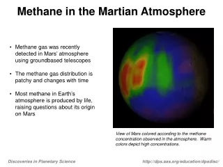
Martian atmosphere in short • Pressure = 6mbar , CO2 @ 95 % (varies with season since atmosphere condenses on the ground) • Mean Surface Temperature = -50°C • Low water vapor content = several tens of micrometers in the atmosphere, but large surface reservoirs (polar caps) • Suspended Particles ( ~ 0.2) : • Dust from the regolith: strong heating power (like desert dust) • Global dust storms ( ~ 5-10) • Ice crystals (H2O, CO2): from condensation (cirrus type) • Earth-like Circulation: • Hadley Cell @ solstices • Strong signal of stationary and transient waves at mid-to-high latitudes in fall/winter
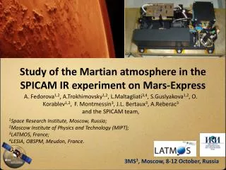
MARS-Express • SPICAM is a one of seven instruments onboard of Mars-Express. • UV spectrometer (118-320 nm) • IR spectrometer (1-1.7 µm; 0.7 kg) • It was inserted into Mars orbit on 25 December 2003. • 4.5 Martian Years of observations: from MY26, Ls 330 (January 2004) to MY 31, Ls 200 (September 2012) • The possibility of continuous study of the atmospheric processes for a long period of time
SPICAM IR – AOTF spectrometer: O21Dg Spectral range: 1-1.7 µm Resolving power: 2000 Spectral resolution: 3.5 cm-1 0.5-1.2 nm FOV nadir: 1° solar occultation: ~0.07° Different observation modes • Nadir viewing (day side) • H2O abundance at 1.38 μm • H2O andCO2 ices • O2 dayglow • Solar occultation • CO2, aerosols, H2O • Limb • Airglow in IR (O21Δg 1.27 μm) • aerosols CO2 ice H2O ice H2O
SPICAM IR nadir measurements Monitoring of Water vapour (2004-2011)
The Current Picture of water vapor cycle • The first observations of water vapour cycle • MAWD/Viking (1977-1979) • The Global asymmetry of present Mars climate • The Northern summer is in 6 times more water than in the southern summer • Only 10-20 precipitated μm corresponds to 1-2 m3of ice! • TES / Mars Global Serveyor (1999-2004) • The reference map of water vapor seasonal cycle for the General Circulation modeling. • The asymmetry is changed. • Interannual variations of water vapor • Studies and modeling of water cycle : Davies [1981], Jakosky [1983], Haberle & Jakosky [1990], Houben et al. [1997], Richardson & Wilson [2002]; Montmessin et al., 2004; Forget et al., 2006; Montmessien et al., 2007 etc. • Transport of water between hemispheres • The role of water clouds in the hemispheric asymmetry (Montmessin et al., 2004) • The example: the role of transport in the deposition of water in the polar caps: perennial water ice at the south pole of Mars could have a precession-controlled mechanism. The GCM shows that 21,500 years ago, when perihelion occurred during northern spring, water ice at the north pole was no longer stable and accumulated instead near the south pole with rates as high as 1 mm yr-1 (Montmessin et al., 2007)
WATER IN MARS ATMOSPHERE: RECENT DATA SETS • The search of interannual variability • Search of daily and spatial variations, condensation and evaporation processes • Mars-Express and MGS experiments can’t give an information about daily variability but can give information about the interannual and spatial variations • Different measurements from 1977 MAWD, 1999 TES, and 2004 Mars-Express, 2006 MRO. Key to a long-term interannual variability? BUT Mars-Express has demonstrated that different measurement methods can’t be used for long-term interannualcomparison The simultaneous observations of water vapor by different spectroscopic instruments on MEX from near IR to thermal range shows a different results (Korablev et al., 2006)
Retrieval of water vapour in Martian atmosphere (SPICAM) • Near IR range (1.38 μm band of H2O) is sensitive to multiple scattering by aerosols in the atmosphere Dust and ice clouds account for MY27-30 (THEMIS/Mars-Odysseydust and ice data with correction) Numerical technique for radiative transfer modeling in the dusty atmosphere (SHDOM) • Uniform mixing of H2O in the atmosphere (up to the saturation level) is assumed • An important issue is an accurate solar spectrum (Fiorenza and Formisano, 2005), with MAWD data correction . • Spectroscopicdatabase: HITRAN 2004-2008 • Liny-by-line calculations • Martian Climate Database V4.3 for temperature-pressure profiles • To minimize a noise SPICAM spectra were averaged by 10 spectra for a fitting Dustopticaldepthfrom THEMIS (Mars Odyssey) 1075 cm-1 and 825 cm-1 (M. Smith, 2009) SPICAM spectrum
Influence of dust account on the retrieval procedure Water vapour with dust account H2O, pr.mm Dust optical depth for 1,38 mkm (“Dust” - ”No dust”) % Dustsinglescatteringalbedow = 0.971; Asymmetryfactor g=0.63
A seasonal map of the H2O distribution by SPICAM H2O, pr.mm MY27 MY27 MY28 MY28 MY29 MY30 Ls
Comparison ofMAWD (1977-1979)TES (1999-2004)SPICAM (2004-2009) • The recalculation of MAWD/Viking 1 and 2 measurements in the same 1.38 μm with modern climate database (GCM 2005) and spectroscopic dataset (HITRAN 2008) • A good agreement with SPICAM measurements in the same 1.38 μm band
Annual water vapour cycle by SPICAM IR All years together H2O, pr.mm Example of water vapour loss during global dust storm at MY28 (seasonal dependence for H2O averaged on latitude stripe (-45:-55)) MY27 1 km3 of ice MY28 Summary • Good dataset of four Martian years for further analysis • “Nothing” else to add to the retrieval algorithm • New solar spectra, resulted in more then 10 % increase of water vapour abundance for polar cap, and up to 20% increase for other areas. • For the first time water vapour map taking into account dust-clouds scattering, to be compared with GCM and other instruments results.
SPICAM IR limb measurements O2 nightglow on MARS (2010-2012)
The O2 dayglow in 1.27 µmon Mars The dayside The O2 emission at 1.27 μm is produced by UV dissociation of ozone O3 + hn O(1D) + O2(a1Dg) 220 nm< l < 320 nm The emission was predicted after the ozone discovery in atmosphere of Mars in spectra recorded by UV spectrometer onboard of Mariner-7 (Barth, 1971). For the first time the emission was detected by Noxon et al. (1976) by means of ground-based telescopes. The maximum values observed in the early spring in both hemispheres are closer to polar regions, reach 30 MR, and its variations reflect variations of the ozone abundance in the atmosphere. Seasonal distribution from January 2004 (Ls=330o) to May 2006 (Ls=50o) Deactivation of the emission: 1) The emission at altitudes >20-25 km O2(a1Dg) O2(X3Sg) + hn (t ~ 4566 s ) 2) Deactivation through collision with CO2CO2(<20 km) O2(a1Dg) + CO2 O2(X3Sg)+ CO2 (k2~ 10-20cm3 s-1)
The nightglow О2 (а1Δg) 1.27 μm on Venus and Mars The O2 emission is produced by oxygen recombination O+O+CO2 O2(a1Dg)+CO2 Venus • The O2 emission was known for a long time • The oxygen emission at 1.27 μm at the night side of Venus is a product of atomic oxygen recombination that in turn is a product of photolysis of CO2 on the dayside andtransfers to the nightside by global circulation in the upper mesosphere and thermosphere of Venus which causes the gas motion from subsolar to antisolar point. Mars • The O2 emission was not detected directly up to 2010 • Atomic oxygen which participates in the reaction, is formed on the dayside of Mars as a result of CO2 photodissociation by solar UV radiation with a wavelength λ <207.5 nm and transported on the night side by the subsolar-antisolar circulation. The transport to the winter polar region is performed by the Hadley meridional cell. (Krasnopolsky, Icarus, 2004)
First detection on Mars in 2010 1) Detection of the O2 nightglow on Mars in 2010 in the OMEGA experiment on Mars-Express (Gondet et al., 2010; Bertaux et al., 2011,2012) There were three detections of the O2 nightglow on limb at the South and North Poles. The vertical emission intensity is 0.24MR 2) Observations of the O2 nightglow on Mars in 2010-2012 by CRISM experiment on MRO (Clancy et al., 2011, 2012) Since July of 2009, the Compact Reconnaissance Imaging Spectrometer for Mars (CRISM) onboard the Mars Reconnaissance Orbiter (MRO) has obtained limb scans over two orbits at solar longitude (Ls) intervals of ~30°. The O2 nightglow
O2 nightglow with SPICAM IR • This emission is an effective indicator of downward flow of air from the altitudes where the CO2photodissociation occurs (i.e. above 70 km). The intensity of the nightglow emission and the altitude of the nightglow layer are controlled by wind magnitudes and eddy diffusion , the key chemical reaction rates. • Since 2010 the OMEGA/MEX does not operate in this spectral range SPICAM IR • Good points: • A campaign of nightglow observations by SPICAM has begun from July 2010 • A new command has been used with a maximal integration time of one spectral point 11.2 ms (5.6 ms is a standard for dayside nadir and solar occultations). One ‘window’ in the spectral range of 1260-1280 nm. 2 sec for one spectrum • IR channel of SPICAM/MEX is turned on now during stellar occultations in 2011-2012 and we hope during night limb from summer 2012. • Bad points: • low vertical distribution of SPICAM with FOV of 1o, about 20 km at limb near a pericenter of orbit • Low sensitivity is not enough for nadir measurements – only limb measurements can be done
First observations (2010), MY30, Ls 150-160, the South Pole Vertical distribution of the O2 (a1Δg) volume emission rate in MR/km can be retrieved from the slant emission. • Tikhonov regularization • the Richardson-Lucy algorithm to deconvolve FOV of SPICAM • an inversion of the O2 volume emission rate in MR/nm for both deconvolved profiles of slant emission and profiles with the SPICAM original resolution • First results for the South Pole: • Vertical resolution for the observations varies from 20 to 35 km. Deconvolution with the FOV was necessary. • Altitude of a peak of the O2 slant emission varies from 37 to 47 km
The Martian general circulation model by LMD (LMDGCM, Lefevre et al., 2004; Millour et al., 2008; version 2012) • a new Martian general circulation (version 2012) • Atmospheric circulation, photochemical cycle, upper atmosphere processes and ionosphere • Plenty of improvements • including Improved Dynamics, Convection and Turbulence Model, Improved “dust model” to simulate observed Martian years (MY24 – MY30), IR and solar wavelength radiative effects of clouds, Improved cloud microphysics etc • A new model well reproduce now • the current MEX and MRO observations
Comparison of the O2 nightglow with the LMD GCM (Lefevre et al., 2004; Millour et al., 2008; version 2012) Black - SPICAM observations; Red - OMEGA data Blue – GCM model (dashed blue – convolved with SPICAM vertical resolution) • the altitude of the nightglow maximum for volume emission rate varies from 45 to 55 km, which corresponds on average the model values. • The vertically integrated emission rate is in 2 times lower than in the model • – more intense transport?
Vertical distribution of the atomic oxygen O + O +CO2 O2(a1Dg)+CO2 (1) Important issue: the oxygen photochemistry controls the energy budget in the 70 to 130 km altitude range. Atomic oxygen is known to have an important effect on the CO2 15-μm cooling. The underestimation of O content would yield an overestimation of the temperature in the GCM modeling. Assuming the vertical distribution of O2(a1Δg) is preliminary controlled by photochemistry. Using appropriate reactions, the equilibrium equation for O2(a1Δg) could be written as: k1 is the rate coefficient of reaction (1), β is the effective yield; k2is thedeactivation rate; τ is radiative lifetime of the excited state The steady state is reached, when photochemical equilibrium exists: The resulting formula for atomic oxygen:
Oxygen profiles and comparison with the GCM Solid lines: observations Dashed lines: LMD GCM modeling The estimated density of oxygen atoms at altitudes from 50 to 65 km varies from 1.5 1011 to 2.5 1011 cm-3 As the basic values we have taken: 1) the kinetics rate of reaction k1(T) = 9.46 × 10⁻³⁴ exp(485/T)cm6 molecule-1 seс-1 (NIST dataset) , 2) the effective yield β =0.75 3) deactivation rate k2=10-20 cm3 molecule-1 seс-1 4) radiative lifetime of the excited state τ =4470 sec. 5) Temperature and atmospheric density vertical profiles were are taken from the LMD general circulation model.
The O2 nightglow observations (2011-2012) • 64 observations (from orbit 8302 to 10642) with the O2 nightglow detected at limb for the North Pole from Ls 250 to Ls 360 and the South Pole from Ls 0 to 120. • Plenty of observations with vertical resolution better than 40 km • The black points are indicated emissions detected at limb • Detection at low latitudes is the O2 day-side afterglow.
Vertical profiles of the O2 emission • Emission peak at 35-42 km for the North Pole and 45-50 km for the South Pole • The emission is more intense for the North Pole
Seasonal distribution of O2 for the South and North Poles Comparison with the GCM O2-O MR The vertically integrated emission rate is totally lower than in the model but the South Pole emission shows more discrepancies The maximum of emission is shifted for the season compared to the GCM model
The temperature and CO2 density from UV stellar occultations Simultaneous observations of atmospheric density The South Pole The South Pole Ls 115-160 • Warming of the middle atmosphere 40-70 km is more strong (on 20-30K) • The atmospheric downwelling circulation over the Pole, which is part of the equator-to-pole Hadley circulation is more strong than expected? • The same results by MCS/MRO McCleese et al.,2008. Not completely improved by the model? • The cold layer at 105 km • The density is much higher The North Pole The North Pole Ls 265-275 • Good agreement for density • Warming in the middle atmosphere is well reproduced • Possible cold layer at 120 km
Conclusions • SPICAM IR on MEX is a small instrument performing observations of the Martian atmosphere: • Mapping of water vapor, search of interannual variability • Good dataset of four Martian years for further analysis • The study of the O2 nightglow as a tracer of polar dynamics • The estimated density of oxygen atoms at altitudes from 50 to 65 km varies from 1.5 to 2.5 1011 cm-3. • The South Pole: the GCM model does not well reproduce the emission, atmospheric density and temperature profiles in the South Pole night. The North Pole: a good agreement with the model • The differences may reflect the current uncertainties in the kinetics of the production of O2(a1Δg), or can be due to an inaccurate downward transport of O atoms by the GCM in the polar night region (especially for the South Pole). • Mapping of O2dayglow (a tracer of ozone on Mars) • Validation of Martian GCM with photochemisty, anticorrelation with water vapour • Validation of kinetic parameters • Vertical distribution of water vapor form solar occultation on Mars • Transport of water, condensation processes • Supersaturation has been detected during the northern spring (Maltagliati et al., 2011) • 5) Dust and water ice clouds studies from solar occultation • Seasonal changes of vertical distribution and particles sizes • Impact on the atmospheric heating in the middle atmosphere