Understanding Terrestrial Carbon Sinks: Variability, Location, and Future Changes
This study aims to explore significant scientific questions surrounding terrestrial carbon sinks, including their existence, locations, interannual variability causes, and potential changes over time. It emphasizes the need for a comprehensive approach that incorporates regional to continental studies, investigates the intersection of climate variability and biomes, and accounts for human land use and natural disturbances. Through methodologies such as flux tower upscaling and inversion modeling, we seek to enhance our understanding of ecosystem-atmosphere CO2 exchanges, informing conservation efforts and carbon management strategies.


Understanding Terrestrial Carbon Sinks: Variability, Location, and Future Changes
E N D
Presentation Transcript
Overarching scientific questions • Why does this terrestrial carbon sink exist? • Where is it located? • What is the cause of the large degree of interannual variability? • How is this terrestrial sink likely to change with time?
Need for regional to continental studies • The intersection of climate variability and biome is regional. • Political units are regional to continental. (carbon cycle manipulation, emission credits) • Human land use activities and natural disturbance patterns are regional.
Motivation I What is and what governs ecosystem-atmosphere exchange of CO2 on spatial scales of geopolitical and bioclimatological relevance?
Motivation II What is and what governsthe interannual variability in ecosystem-atmosphere exchange of CO2 on spatial scales of geopolitical and bioclimatological relevance?
Flux: R, NEE, GEP Climate variables (x, y) Flux tower upscaling hypothesis Each point ~ (1 km)2 Flux = ax + by + c, interpolate fluxes over ~ (1000 km)2 Segregate further by ecosystem characteristics? Stand type (conifer, deciduous, grass, crop) Stand age (young, mature, old)
s(flux) = flux – mean flux Climate variables (x, y) Flux tower upscaling hypothesis II – interannual variability Each point ~ (1 km)2 s(flux) = ax + by + c, interpolate interannual variability in fluxes over ~ (1000 km)2 Ecosystem fluxes respond similarly to climate variability across a wide range of forest types and ages(?)
Air Parcel wind wind Sinks Air Parcel Air Parcel Sources Sample Sample Inverse Modeling of CO2 Changes in CO2 in the air tell us about sources and sinks
Complementary nature of inversion downscaling and flux tower upscaling Inversion downscalingFlux tower upscaling Excellent spatial Intrinsically local integration measurements. Strong constraint on Difficult to upscale flux flux magnitude magnitudes. Variability easier. Poor temporal Excellent temporal resolution resolution Limited mechanistic Strong mechanistic understanding. understanding
Chequamegon Ecosystem-Atmosphere Study (ChEAS) region flux towers U. Minnesota, Penn State, U. Toledo, NOAA-CMDL, U. Michigan, USDA-FS Support: DoE, NSF, USDA, NASA, NOAA
WLEF CO2 flux and mixing ratio observatory Photo credit: UND Citation crew, COBRA NOAA CMDL Penn State U. Minnesota USDA-FS Support from: NOAA DoE WLEF tall tower (447m) CO2 flux measurements at: 30, 122 and 396 m CO2 mixing ratio measurements at: 11, 30, 76, 122, 244 and 396 m
ChEAS land cover/vegetation Green = upland forest Purple = forested wetland Blue = open water Yellow = agriculture or grassland
Why is the ChEAS region unique? • Existing flux tower network, including old growth, wetlands, world’s only tall tower with CO2 fluxes • Existing “top-down” efforts • Ring of towers: Davis, Richardson, Denning • COBRA regional: Lin, Gerbig, Wofsy • Simple ABL budgets approaches: Helliker, Berry, Bakwin • NOAA CMDL tall tower and aircraft sampling site • Extensive paleoecological history and relatively simple land use history • Simple topography, light population density • Complex forest mosaic including human management, extensive wetlands. • Ecosystem intersection nearby – temperate forest, boreal forest, agriculture/prairie – vulnerable to climate change
What issues general to the NACP can be addressed via a ChEAS regional intensive? Regional flux estimate methodology • Downscaling: The techniques needed to determine regional carbon fluxes via atmospheric budgets are still experimental. Existing work is advancing this methodology in ChEAS. • Upscaling: The measurements and models needed to upscale fluxes to regional scale are uncertain. The density of flux towers, simple topography, complex forest mosaic and tall flux tower in ChEAS collectively present a unique site for upscaling experiments. • Evaluation: Verifiable regional flux estimates (at least two independent methods) have yet to be constructed. This can be done at ChEAS. • Regional mechanistic understanding: The mechanisms that govern interannual and decadal-scale forest-atmosphere carbon exchanges remain uncertain. This mechanistic understanding is limited by the lack of regional flux measurements that can accurately resolve seasonal-scale fluxes yet be deployed for several years. This can be achieved at ChEAS.
Flux tower up-scaling with simultaneous top-down constraints Continent: Map biomes and climate, model fluxes N. American [CO2] Region: Map ecosystem variables, model fluxes N. Wisconsin [CO2] WLEF tower Forest: Map ecosystem variables, model fluxes Stand: Eddy covariance flux towers Within stand: biometric data, chamber fluxes
What more region-specific scientific issues can be addressed via a ChEAS regional intensive? • What is causing a net source of carbon dioxide to the atmosphere at the forest (WLEF) scale? • Forest management practices? • Climate change and wetland drying? • Are forest-scale (WLEF) fluxes representative of the region? What is preventing simple regional flux-tower up-scaling from being successful? • Wetland margins? • Forest management/disturbance history? • Systematic errors in tower flux measurements? • Find general guidance for up-scaling methodology
What more region-specific scientific issues can be addressed via a ChEAS regional intensive? • What is causing observed interannual variability in carbon fluxes? Can consistent mechanistic explanations be found across the plot, stand, forest and regional scales? • Methane and wetlands: • How is the methane/CO2 flux ratio linked to climate and the hydrological budget? • Are the combination of methane and co2 fluxes in the region a net source or sink for GHG forcing? • How does management and climate influence this net GHG source/sink?
What additional resources are needed for a ChEAS region intensive? • Methane measurement infrastructure • Continued support for the existing flux tower network • Additional emphasis on: • Remote sensing and advanced ecosystem modeling • Forest inventory and disturbance history studies • Longer-term support of a regional mixing ratio observing network, and associated inverse modeling. • Support for integration of existing measurements
ChEAS flux tower array Yi et al, 00 Berger et al, 01 Davis et al, 03 Ricciuto et al, B51 Mackay et al, 02 Mackay et al, H29 Ewers et al, 02 Ewers et al, H30 Forest-scale flux: WLEF tower, 1997-present Dominant stand types and flux towers: Northern Aspen Forested Conifer hardwood wetland young old mature Willow Creek (UMBS) Lost Creek Chen B 2000-present 1999-present 2001-present 2002-present Bolstad et al, in press Cook et al, in prep Chen A 2002–present Sylvania 2002-present Desai et al, in prep Desai et al, B52D-04 Chen mobile Chen mobile 2003 2002
Testing the upscaling hypothesis: Regional clusters of flux towers • Can fluxes be up-scaled from stand to forest or region? • Clusters can isolate the role of ecosystem characteristics via identical climate across sites. • What must be measured and mapped for flux upscaling?
NEE of CO2 at WLEF(forest scale) • The region is a net source of CO2 to the atmosphere. • Interannual variability is significant – resolved by the measurements. • Interannual variability is caused by changes in the timing of leaf-out, and correlated with changes in soil moisture.
Chamber respiration fluxes Table 4. Estimated annual respiration for the whole ecosystems and components, 1999-2002. All rates are reported in Mg C ha-1 yr-1. Bolstad et al, in press.
ChEAS upscaling test results • Climate alone does not explain ChEAS CO2 fluxes. • The WLEF footprint is a source of CO2 to the atmosphere. • drying wetlands? • disturbance/management? • WLEF fluxes cannot be explained as a linear combination of Lost Creek and Willow Creek fluxes. • aspen? conifers? WLEF footprint dissimilar? systematic errors that differ among flux towers? • Soil + leaf + stem respiration is similar in aspen and northern hardwoods in the Willow Creek area. • WLEF high respiration rate due to coarse woody debris?
Interannual variability upscaling results • ChEAS annual fluxes (R, GEP, NEE) are moderately coherent across ChEAS sites, 2000-2001. (Caterpillars, not climate?). • ChEAS chamber and tower R fluxes show similar variability, 2001-2002, across sites. (2001 high flux, 2002 low flux). s(WLEF) = a*s(W Creek) + b*s(L Creek)? 3. Continental scale fluxes are very coherent, spring 1998, and linked to [CO2]! (Butler et al, in prep) An extreme climatic event.
ChEAS Regional Flux Experiment Domain = 40m Sylvania flux tower with high-quality standard gases. = LI-820 sampling from 75m above ground on communication towers. = 447m WLEF tower. LI-820, CMDL in situ and flask measurements.
ChEAS Regional Flux Experiment • Derive daytime and daily seasonal fluxes using regional atmospheric inversions and relatively inexpensive in situ CO2 sensors. • Overarching goal – evaluate/merge multiple approaches of studying terrestrial fluxes of CO2. • Merge flux-tower based upscaling with downscaled inversion methodology. Regional integration and mechanistic interpretation. • Determine interannual variations in seasonal fluxes on a regional basis. Again, integrate with regional flux measurements/mechanistic interpretations. • If possible, derive net annual fluxes. Spatial resolution is limited by the magnitude of the annual signal.
Time scale Daytime Diurnal Annual Flux magnitude 1 to 10 mmol m-2 s-1 1 to 4 gC m-2 d-1 ~ 1 gC m-2 d-1 Mixing depth 1 to 2 km 1 to 2 km ~10 km Advection time ~10 hours ~24 hours Advection distance ~180 km (half ring) ~400 km (full ring) 400 km (full ring) Change in ABL CO2 1 to 5 ppm 2 to 5 ppm ~0.2 ppm Expected Regional Mixing Ratio Differences (Winter to Summer)
Planned continental CO2 network:Selection of new sites based on optimization study, Skidmore et al, and plans for a Midwest regional intensive
Spatial coherence of seasonal flux anomalies A similar pattern is seen at several flux towers in N. America and Europe. Three sites have high-quality [CO2] measurements + data at Fluxnet (NOBS, HF, WLEF). The spring 98 warm period and a later cloudy period appear at all 3 sites.