Multi-State Modeling of Mortgage Insurance: Insights from Actuarial Research
270 likes | 391 Vues
This presentation explores the complexities of modeling mortgage insurance as a multi-state process, focusing on the risks associated with lenders mortgage insurance (LMI). Highlighted are the unique characteristics of LMI policies, premiums, and claims experience, which depend on economic variables. The use of Generalized Linear Models (GLMs) to understand claims behavior and forecast future liabilities is discussed. Key predictors include policy-specific and external economic factors. The importance of accurate modeling for predicting claims and ensuring financial stability in the mortgage sector is emphasized.

Multi-State Modeling of Mortgage Insurance: Insights from Actuarial Research
E N D
Presentation Transcript
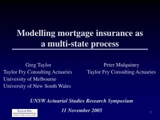
Modelling mortgage insurance as a multi-state process Peter Mulquiney Taylor Fry Consulting Actuaries Greg Taylor Taylor Fry Consulting Actuaries University of Melbourne University of New South Wales UNSW Actuarial Studies Research Symposium 11 November 2005
Mortgage insurance (aka Lenders mortgage insurance (LMI)) • Indemnifies lender against loss in the event of default by the borrower when collateral property is sold • Loss would occur if sale price less associated costs is insufficient to meet outstanding loan principal
Mortgage insurance (cont’d) • Policies have relatively unique properties • Single premium but multi-year coverage • Claims experience influenced by variables related to housing sector of economy • Claim occurs at a defined sequence of events
Earning of premium • Accounting Standard requires that earning of premium be proportionate to incidence of risk • Typical situation • Premium is earned in fixed percentages over the years of a policy’s life • E.g. 5% in Year 1, 15% Year 2, etc • True incidence of risk over lifetime of a cohort of policies will vary with economic conditions • Downturn in house prices likely to generate claims
Literature survey • Taylor (1994): Modelled claims experience with a GLM with external economic variables as predictors • Ley & O’Dowd (2000): Extended GLM to allow for changes in LMI market and products • Driussi & Isaacs (2000): Overview of LMI industry, less concerned with modelling. Contains useful data • Kelly & Smith (2005): Stochastic model of external economic predictors
Multi-state process leading to a claim Healthy Cured Property in possession In arrears Loan discharged Borrower’s sale Property sold Claim
Transition matrix • Each distinct probability requires a separate model
Required models • Probability Healthy In arrears • Probability of cure of arrears • Probability In arrears PIP • Probability PIP Sold • Probability Sold Claim • Distribution of claim sizes • The case [In arrears Sold] may be treated as: In arrears PIP Sold Nil duration
Structure of sub-models – transition probabilities • GLMs for all 6 sub-models • Five of them are probabilities Y(m)ij ~ Bin [1,1 - exp {u(m)ij log [1 - p(m)ij]}], m=1,…,5 where • Y(m)ij is binomial response of the i-th policy in the j-th calendar interval under the m-th model • e.g. the transition Healthy In arrears • p(m)ij is the associated probability • u(m)ij is the time on risk of the relevant transition logit p(m)ij = Σk β(m)k xijk with • xijk predictors • β(m)k their coefficients
Structure of sub-models – claim size Y(6)ij ~ EDF(μij,q) log μij = Σk β(6)k xijk E[Y(6)ij] = μij Var[Y(6)ij] = (φ/wij) μijq • We found q=1.5 satisfactory • Right skewed • But shorter tailed than Gamma
Predictors • Several categories • Policy variables (specific to individual policies) • Static, e.g. date of policy issue, Loan-to-valuation ratio (LVR) • Dynamic, e.g. number of quarters since transition into current status • External economic variables (common to all policies), e.g. interest rates, rates of housing price increases • Manufactured risk indicators (derivatives of the previous categories)
Manufactured risk indicators – an example Potential claim size = Amount of arrears less Principal repaid less Original loan amount X [Housing price growth factor X (1-q) / LVR -1] where • Housing price growth relates to period from inception to the current date • q = proportion of property value lost in deadweight costs on sale Growth in borrower’s equity
Predictors (cont’d) • There may be many potential predictors available in the data base, e.g. • State of Australia • Issue quarter • LVR • Stock price growth • etc • We found a total of more than 30 statistically significant predictors over the 6 models • Many appear in more than one model • More than 20 in one of the models
Forecast claims experience • We take the fitting of the GLM sub-models to claims experience as routine • No further comment on this • Conventional form of forecasting future claims experience consists of plugging parameter estimates into models over future periods • This procedure is undesirable on two counts • Not feasible computationally • Produces biased forecast
Computational feasibility • Example of evolution of a claim • Too many combinations for feasible computation
Forecast bias • Forecast liability (outstanding claims or premiums) takes form L* = ∑ i,j L(j)i(β, x*ij) where • L(j)i(.,.) = simulated liability cash flow of policy i in future calendar quarter j • β = parameter estimates • x*ij = future values of predictors
Forecast bias (cont’d) • Forecast liability (outstanding claims or premiums) takes form L* = ∑ i,j L(j)i(β, x*ij) x*ijT = [ξ*iT,ζ*ijT,z* ijT] Static policy variables (non-stochastic) External economic variables (stochastic) Dynamic policy variables (non-stochastic)
Jensen’s inequality • Jensen’s inequality. Let f be a function that is convex downward. Let X be a random variable. Then • E[f(X)] ≥ f(E[X]) • with equality if and only if either • f is linear; or • the distribution of X is concentrated at a single point
Jensen’s inequality • Jensen’s inequality. Let f be a function that is convex downward. Let X be a random variable. Then • E[f(X)] ≥ f(E[X]) • with equality if and only if either • f is linear; or • the distribution of X is concentrated at a single point y=f(x) E[f(x)] f(E[X])
Forecast bias (cont’d) L* = ∑ i,j L(j)i(β, x*ij) = ∑ i,j L(j)i(.,.,., z*ij) [z stochastic] • L* is convex downward in some of the components of z*ij • E.g. z*ijk = rate of increase of house price index • By Jensen’s inequality • E[L*] ≥ ∑ i,j L(j)i(.,.,., E[z*ij]) • Plugging expected values of external variables into forecast leads to downward bias • This result has recently been observed empirically by Kelly and Smith (2005) • For other lines of business, this is usually not significant because the external variables have much lower dispersion (e.g. superimposed inflation)
Forecast error • Forecast model is fully stochastic • Forecast error (MSEP) can be estimated, consisting of: • Specification error • (Model) parameter error • Process error • Predictor error • Due to future stochastic variation of predictors
Estimation of forecast error • By means of an abbreviated form of bootstrap • We refer to it as a fast bootstrap • Conventional bootstrapping (re-sampling) is not computationally feasible
Fast bootstrap Just sample assuming normally distributed with model estimates of mean and standard error
Computation L* = ∑ i,j L(j)i(β, x*ij) • Need to simulate for: • All values of i (=policy), j (=future period) • All stochastic components of x*ij • This produces: • Central estimate • Process error • Then need to re-simulate for each drawing of pseudo-parameters • This produces: • Parameter error • Stochastic predictor error
References • Driussi A and Isaacs D (2000). Capital requirements for mortgage insurers.Proceedings of the Twelfth General Insurance Seminar, Institute of Actuaries of Australia, 159-212 • Kelly E and Smith K (2005). Stochastic modelling of economic risk and application to LMI reserving. Paper presented to the XVth General Insurance Seminar, 16-19 October 2005 • Ley S and O’Dowd C (2000). The changing face of home lending. Proceedings of the Eleventh General Insurance Seminar, Institute of Actuaries of Australia, 95-129 • Taylor G C (1994). Modelling mortgage insurance claims experience: a case study. ASTIN Bulletin, 24, 97-129.
