Download
1 / 33
330 likes | 437 Vues
Efficient Simulations of Gas-Grain Chemistry Using Moment Equations. M.Sc. Thesis by Baruch Barzel preformed under the supervision of Prof. Ofer Biham. Complexity in the Universe. Complexity in the Universe. Horse-Head Nebula. The Interstellar Clouds (ISC). The Interstellar Clouds.

E N D
Efficient Simulations of Gas-Grain Chemistry Using Moment Equations M.Sc. Thesis by Baruch Barzel preformed under the supervision of Prof. Ofer Biham
Complexity in the Universe Horse-Head Nebula
The Interstellar Clouds • Gas Temperature: 50 -150 K • Density: ~10 -1000 (atoms cm-3) • Molecular and atomic H
Complex Molecules Star Formation The Role of H2 H2 Complexity
Observed Production Rates in ISC: RH ~ 10-15 (mol cm-3s-1) 2 The H2 Puzzle H2 Production in the gas phase: H + H → H2 Gas-Phase Reactions Cannot Account for the Observed Production Rates
The Interstellar Dust Grains • Composition: • Carbons, Silicates, Olivine, H2O, SiC • Temperature: ~5-20 K • Size Range: • 10-6-10-3 (cm) → 100-108 sites • Activation Energies: (meV)
d‹NH› dt = FH - WH‹NH› - 2AH‹NH›2 -E0 -E1 kBT kBT WH = n e RH= AH‹NH›2 (mol s-1) AH = (1/S)n e 2 Incoming flux Recombination Desorption The Rate Equation The Production Rate of H2 Molecules:
d‹NH› dt = FH - WH‹NH› - 2AH‹NH›2 When the Rate Equation Fails Mean-field approximation • Neglects fluctuations • Ignores discretization Not valid for small grains and low flux
Flux term: FH[PH(NH-1) - PH(NH)] Desorption term: WH[(NH+1)PH(NH+1) - NHPH(NH)] FH WH AH Reaction term: AH[(NH+2)(NH+1)PH(NH+2) - NH(NH-1)PH(NH)] Probabilistic Approach
= FH[PH(NH-1) - PH(NH)] + WH[(NH+1)PH(NH+1) - NHP(NH)] + AH[(NH+2)(NH+1)PH(NH+2) - NH(NH-1)PH(NH)] dPH(NH) dt RH=AH (‹NH2› - ‹NH›) S ‹NH›=S NHPH(NH) 2 NH= 0 The Master Equation
FH = 10-10S(atoms s-1) E0 = 22 E1=32 (meV) Tsurface= 10 K RH vs. Grain Size 2
1 3 2 H H2 H2O OH OH O O2 Complex Reactions The parameters: Fi ; Wi ; Ai (i=1,2,3)
= F1 - W1‹N1› - 2A1‹N1›2 - (A1+A2)‹N1›‹N2› - (A1+A3)‹N1›‹N3› d‹N1› dt d‹N2› dt d‹N3› dt =F2 – W2‹N2› - 2A2‹N2›2 - (A1+A2)‹N1›‹N2› = F3 - W3‹N3› - (A1+A3)‹N1›‹N3›+(A1+A2)‹N1›‹N2› The Rate Equations
P(N1,N2,N3) = S Fi[P(…,Ni-1,…)-P(N1,N2,N3)] +S Wi[(Ni+1)P(..,Ni+1,..)-NiP(N1,N2,N3)] +S Ai[(Ni+2)(Ni+1)P(..,Ni+2,..)-Ni(Ni-1)P(N1,N2,N3)] S + (A1+A2)[(N1+1)(N2+1)P(N1+1,N2+1,N3-1)-N1N2P(N1,N2,N3) S + (A1+A3)[(N1+1)(N3+1)P(N1+1,N2,N3+1)-N1N3P(N1,N2,N3) 3 i=1 3 i=1 2 i=1 The Master Equation
P(N1,N2,N3) = S Fi[P(…,Ni-1,…)-P(N1,N2,N3)] +S Wi[(Ni+1)P(..,Ni+1,..)-NiP(N1,N2,N3)] +S Ai[(Ni+2)(Ni+1)P(..,Ni+2,..)-Ni(Ni-1)P(N1,N2,N3)] S + (A1+A2)[(N1+1)(N2+1)P(N1+1,N2+1,N3-1)-N1N2P(N1,N2,N3) S + (A1+A3)[(N1+1)(N3+1)P(N1+1,N2,N3+1)-N1N3P(N1,N2,N3) 3 i=1 3 i=1 2 i=1 Rij = (Ai+Aj)‹NiNj› Rii = Ai(‹Ni2› - ‹Ni›)
The Rate vs. The Master Rate equations: • Mean field approximation • High efficiency • Not reliable for surface reactions (at low coverage) Master equation: • Microscopic probability distribution • Accurate model of grain surface reactions • Low efficiency (exponential growth) • Hard work
8 ‹NHk› = SNHkPH(NH) NH=0 ‹NH› = FH + (2AH - WH)‹NH›- 2AH‹NH2› ‹NH2› = FH + (2FH + WH - 4AH)‹NH› + (8AH - WH)‹NH2› - 4AH‹NH3› The Moment Equations After applying the summation:
‹NH1›= PH(1) + 2PH(2) + +kPH(k) ‹NH2›= PH(1) + 22PH(2) + +k2PH(k) ‹NHk›= PH(1) + 2kPH(2) + +kkPH(k) Truncating the Equations PH(NH > k) = 0 1. Set the cutoff 2. Express the (k+1)th moment by the first k moments
‹NH1›= PH(1) + 2PH(2) + + kPH(k) k ‹NH2›= PH(1) + 22PH(2) + +k2PH(k) i=0 ‹NHk›= PH(1) + 2kPH(2) + +kkPH(k) ‹NHk+1› = SCi‹NHi› Truncating the Equations PH(NH > k) = 0 1. Set the cutoff 2. Express the (k+1)th moment by the first k moments 3. Plug into the first k moment equations
‹NH› = FH + (2AH - WH)‹NH›- 2AH‹NH2› ‹NH2› = FH + (2FH + WH - 4AH)‹NH› + (8AH - WH)‹NH2› - 4AH‹NH3› 1. Set the cutoff → k=2 Moment Equations for H2 Production ‹NH3›= 3‹NH2› - 2‹NH› 2. Reduce excessive moments → 3. Plug into the equations…
‹NH› = FH + (2AH - WH)‹NH›- 2AH‹NH2› ‹NH2› = FH + (2FH + WH + 4AH)‹NH› - (4AH + 2WH)‹NH2› ‹NH› = FH + (2AH - WH)‹NH›- 2AH‹NH2› ‹NH2› = FH + (2FH + WH - 4AH)‹NH› + (8AH - WH)‹NH2› - 4AH‹NH3› 1. Set the cutoff → k=2 ‹NH3›= 3‹NH2› - 2‹NH› 2. Reduce excessive moments → 3. Plug into the equations… Moment Equations for H2 Production
H H2 H2O OH O2 OH O The challenge: Reduction of the excessive moments ‹N1aN2bN3c› =SClnm‹N1lN2nN3m› k-1 lmn=0 Moments for Complex Networks The probability: P(N1,N2,N3) The moments:‹N1aN2bN3c› The cutoff: Ni < ki
k-1 ‹N1aN2b› = SN1aN2b P(N1,N2) N1N2=0 V(a,b) P(N1,N2) M(N1,N2,a,b) v = M p k-1 ‹N1aN2b› =SCnm‹N1nN2m› mn=0 Reduction of Excessive Moments The probability: P(N1,N2)
‹N1›, ‹N2›, ‹N3› H H2 ‹N12› H2O OH ‹N22› OH O O2 Setting the Cutoffs ‹N1N2› ‹N1N3› 3 vertices + 2 edges + 2 loops = 7 equations
7 vertices 8 edges 2 loops 17 equations H2CO H3CO OH HCO H O CO H3CO CH3CO + H2O H2CO H2 CO2 + H OH HCO CO2 O2 Multi-Specie Network
Summary • The advantages of the moment equations: • Reliable even for low coverage • Efficient • Linear • Easy to incorporate into rate equation models • Directly generate the required moments • Further applications should be tested.
The moment equations validity - For small grains For large grains Cutoff justified PH(NH) is Poisson Moment equations valid under all circumstances • Second order: (h << 1) • The equations are valid • First order: (h ≈ 1) • Production rate is accurate but population size may deviate Revealing the Trick