4.1 Linear Transformations
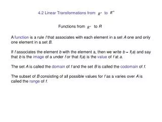
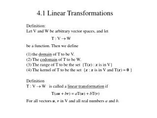
4.1 Linear Transformations. Definition: Let V and W be arbitrary vector spaces, and let T : V W be a function. Then we define the domain of T to be V. The codomain of T to be W. The range of T to be the set {T( x ) : x is in V}

4.1 Linear Transformations
E N D
Presentation Transcript
4.1 Linear Transformations • Definition: • Let V and W be arbitrary vector spaces, and let • T : V W • be a function. Then we define • the domain of T to be V. • The codomain of T to be W. • The range of T to be the set {T(x) : x is in V} • The kernel of T to be the set {x : x is in V and T(x) = 0 } Definition T : V W is called a linear transformation if T(au + bv) = aT(u) + bT(v) For all vectors u, v in V and all real numbers a and b.
(2) Differentiation Let C1[a, b] be the vector space of all functions that are continuously differentiable in the interval [a, b], and if we define D( f(x) ) = then this will be a linear transformation from C1[a, b] to C0[a, b] Examples of Linear Transformations • Matrix multiplications • If A is an m×n matrix, then we can use A to define a linear transformation • T : nm • by defining • T(x) = AxT
(3) Integration Let C0[a, b] be the vector space of all functions that are continuous on the interval [a, b] then is a linear transformation. Examples of Linear Transformations (4) Let Pk be the vector space of all polynomials of degree less than or equal to k. If we define T( p(x) ) = xp(x) then T will be a linear transformation from Pk to Pk+1 .
Simple properties of a linear transformation Let T : V W be a linear transformation, then (1) T(0) = 0 (2) if {v1, v2, … , vn} is a basis for V then T is completely determined by the values of T(v1), … , T(vn). (3) if T is a linear transformation from n to m , and A is the associated m×n matrix, then the 1st column of A is T([1, 0, 0, ··· , 0]T), the 2nd column of A is T([0, 1, 0, ··· , 0]T), . . . . . . the nth column of A isT([0, ··· , 0, 1]T),
Fact: If both V and W are finite dimensional vector spaces and B1 = {v1, v2, … , vm } is a basis for V and B2 = {w1, w2, … , wn } is a basis for W then any given linear transformation T : V W can be represented by a n×m matrix whose entries are determined by T(v1) = a11 w1 + a21 w2 + · ·· + an1 wn T(v2) = a12 w1 + a22 w2 + · ·· + an2 wn … …
Given any vector u in V, we can express u = b1 v1 + b2 v2 + · ·· + bm vm hence T(u) = b1 T(v1) + b2 T(v2) + · ·· + bm T(vm) = b1 [a11 w1 + a21 w2 + · ·· + an1 wn] + b2 [a12 w1 + a22 w2 + · ·· + an2 wn] + . . . bm [a1m w1 + a2m w2 + · ·· + anm wn] And since the matrix A = [aij] depends so much on the basis B1 and B2, it is therefore necessary to choose good basis such that the matrix A is as simple as possible, such as upper triangular or even diagonal.
Theorem • If T : V W is a linear transformation then • ker(T) is a subspace of V, • Range(T) is a subspace of W. • Definition • A function T : V W is said to be • one-to-one if T(x) ≠ T(y) whenever x ≠ y • onto if Range(T) = Codomain(T) Theorem For a linear transformations T : V W, T is one-to-one if and only if ker(T) = {0}
The Dimension Theorem for Linear Transformations If T : V W is a linear transformation, then we have dim(ker(T)) + dim(Range(T)) = dim(V) Remark: dim(Range(T)) is also called the Rank of T • Consequences: • If dim(V) < dim(W), then T cannot be onto, • If dim(V) > dim(W), then T cannot be one-to-one, • If dim(V) = dim(W), and T is one-to-one, then T is also onto, • If dim(V) = dim(W), and T is onto, then T is also one-to-one.
2D Geometric Transformations • The most common types of linear geometric transformations are • Rotation (about the origin) • Reflection (about a line through the origin) • Expansion or compression • shear And if a transformation is linear, it can be carried out by matrix multiplications, i.e. Translations are not linear transformations, but we can still perform a 2D transformation with matrix multiplication using a very clever 3D shear. We will see this at the end.
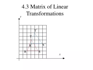
y y x x 2D Geometric Transformations (1) Rotation about the origin by angle in anticlockwise direction.
y y x x 2D Geometric Transformations (2a) Reflection about the x-axis.
y y x x 2D Geometric Transformations (2b) Reflection about the y-axis.
y x 2D Geometric Transformations (2c) Reflection about an inclined line through the origin. y θ x • This reflection can be decomposed into 3 basic operations • rotation about the origin by -θ. • reflection about the x-axis • rotation about the origin by θ.
y x 2D Geometric Transformations (3a) Expansion (or compression) along the x-axis. y x This is an expansion if k > 1, and is a compression if 0 < k < 1.
y x 2D Geometric Transformations (3b) Expansion (or compression) along the y-axis. y x This is an expansion if k > 1, and is a compression if 0 < k < 1.
y x 2D Geometric Transformations (4a) Shear along the x-axis (by the factor of k > 0). y k 1 1 x 1 If k < 0, then the shear is to the other side.
y x 2D Geometric Transformations (4b) Shear along the y-axis (by the factor of k > 0). y 1 1 1 k x If k < 0, then the shear is to the other side.
y x 2D Geometric Transformations (5) Translations – these are not really linear transformations, but y 1 1 1 1 x we can cleverly embed the 2D picture into 3D first, then do a 3D shear, then finally project the result down to 2D. Here are the details:
z y x Shears in 3D
Shears in 3D z y x
y x Shears in 3D z Please note that a shear in 3D along the x or y direction will induce a translation of the plane z = 1 in the corresponding direction
Shears in 3D z Please note that a shear in 3D along the x or y direction will induce a translation of the plane z = 1 in the corresponding direction y x
Shears in 3D z Please note that a shear in 3D along the x or y direction will induce a translation of the plane z = 1 in the corresponding direction y x
z y x Shears in 3D Please note that a shear in 3D along the x or y direction will induce a translation of the plane z = 1 in the corresponding direction
z y x Shears in 3D Please note that a shear in 3D along the x or y direction will induce a translation of the plane z = 1 in the corresponding direction
y project 3D shear embed x 2D Geometric Transformations (5) Translations y 1 1 1 1 x
2D Geometric Transformations Summary In actual practice, we will first embed all 2D graphics into 3D (as in the previous example), then perform all kinds of linear transformations by matrix multiplications. Finally we project the result back down to 2D. For 3D objects, we need to embed them into a 4D space first, and then do the transformation there, hence 4D spaces also have geometric applications. Questions: How do we rotate a 2D object about a point away from the origin? How do we reflect a 2D object about a line not going through the origin?
Inner Products and related topics • Definition • Let V be a real vector space, a function • ·: V×V • is called an inner product in V if it satisfies the following • u· v = v·u • (u + v) · w = u · w + v · w • (ru) · v = r(u · v) • u · uù0, and u · u = 0 if and only if u = 0
(III) Let S = { {an}: is finite} We can define the inner product · as {an} · {bn} = (II) In C0[a, b] (i.e. the vector space of all functions that are continuous on the interval [a, b] ), the inner product is Examples • In n the standard inner product is • (a1 , … , an) · (b1, … , bn) = a1 b1 + … + an bn
Definition A collection of vectors in a vector space V is said to be orthogonal if the vectors are mutually orthogonal. The same set is said to be orthonormal if it is an orthogonal set and each vector in the set has unit length. Examples(I) The standard basis in n is an orthonormal set, e1 = (1, 0, 0, … , 0), e2 = (0, 1, 0, … , 0), … , en = (0, 0, 0, … , 1),
(II) In 8 we also have another not so obvious orthonormal set, and this is used in the JPEG compression standard
(III) In Fourier series, we have the orthonormal set in C0[0, 2π] Theorem If v1, v2, … vm are non-zero orthogonal vectors, then they are linearly independent.
Definition A collection of (column) vectors in n is said to be orthogonal if the vectors are mutually orthogonal. The same set is said to be orthonormal if it is an orthogonal set and each vector in the set has unit length. Definition An n×n matrix is said to be orthogonal if its columns form an orthonormal set
Matrices and Dot products • Let A be an m×n matrix, let B be an n×m matrix, let x be a (column vector in n, and y be a (column) vector in m, then • Ax·y = x · ATy • x · By = BT x · y Theorem If A is an n×n orthogonal matrix, then ATA = In = A(AT) or in other words A-1 = AT
The Gram-Schmidt Process Given a set of n linearly independent vectors v1, v2, … vn , in an inner product space V, this process will construct n linearly independent vectors u1, u2, … un also in V such that (1) span(u1, u2, … un ) = span(v1, v2, … vn ) (2) u1 is “parallel” to v1 Corollary Given any nonzero subspace W of an inner product space V, we can always find an orthonormal basis. In addition, the “direction” of one of those vectors in the orthonormal basis can be predetermined.