Download
1 / 63
640 likes | 854 Vues
The transition to strong convection. Background: precipitation moist convection & its parameterization; Arakawa’s Quasi-Equilibrium postulate (QE); + reasons to care QE in vertical structure The onset of strong convection regime as a continuous phase transition with critical phenomena.

E N D
The transition to strong convection • Background: precipitation moist convection & its parameterization; Arakawa’s Quasi-Equilibrium postulate (QE); + reasons to care • QE in vertical structure • The onset of strong convection regime as a continuous phase transition with critical phenomena J. David Neelin1, Ole Peters1,2, Chris Holloway1, Katrina Hales1, Steve Nesbitt3 1Dept. of Atmospheric Sciences & Inst. of Geophysics and Planetary Physics, U.C.L.A. 2Santa Fe Institute (& Los Alamos National Lab) 3U of Illinois at Urbana-Champaign
The transition to strong convection • Background: precipitation, moist convection and its parameterization; Arakawa’s Quasi-Equilibrium postulate (QE); + reasons to care • QE in vertical structure • The onset of strong convection regime as a continuous phase transition with critical phenomena J. David Neelin1, Ole Peters1,2, Chris Holloway1, Katrina Hales1, Steve Nesbitt3 1Dept. of Atmospheric Sciences & Inst. of Geophysics and Planetary Physics, U.C.L.A. 2Santa Fe Institute (& Los Alamos National Lab) 3U of Illinois at Urbana-Champaign
The transition to strong convection • Background: precipitation, moist convection and its parameterization; Arakawa’s Quasi-Equilibrium postulate (QE); + reasons to care • QE in vertical structure • The onset of strong convection regime as a continuous phase transition with critical phenomena J. David Neelin1,Ole Peters1,2,*, Chris Holloway1, Katrina Hales1, Steve Nesbitt3 1Dept. of Atmospheric Sciences & Inst. of Geophysics and Planetary Physics, U.C.L.A. 2Santa Fe Institute (& Los Alamos National Lab) 3U of Illinois at Urbana-Champaign * + thanks to Didier Sornette for connecting the authors & Matt Munnich & Joyce Meyerson for terabytes of help
Background: Precipitation climatology July January Note intense tropical moist convection zones (intertropical convergence zones) 2 8 16 4 mm/day
Rainfall at shorter time scales Weekly accumulation Rain rate from a 3-hourly period within the week shown above (mm/hr) From TRMM-based merged data (3B42RT)
Convective quasi-equilibrium (Arakawa & Schubert 1974) • Convection acts to reduce buoyancy (cloud work function A) on fast time scale, vs. slow drive from large-scale forcing (cooling troposphere, warming & moistening boundary layer, …) • M65= Manabe et al 1965; BM86=Betts&Miller 1986 parameterizns Modified from Arakawa (1997, 2004)
Background: Convective Quasi-equilibrium cont’d Manabe et al 1965; Arakawa & Schubert 1974; Moorthi & Suarez 1992; Randall & Pan 1993; Emanuel 1991; Raymond 1997; … • Slow driving (moisture convergence & evaporation, radiative cooling, …) by large scales generates conditional instability • Fast removal of buoyancy by moist convective up/down-drafts • Above onset threshold, strong convection/precip. increase to keep system close to onset • Thus tends to establish statistical equilibrium among buoyancy-related fields – temperature T & moisture, including constraining vertical structure • using a finite adjustmenttime scale tc makes a difference Betts & Miller 1986; Moorthi & Suarez 1992; Randall & Pan 1993; Zhang & McFarlane 1995; Emanuel 1993; Emanuel et al 1994; Yu and Neelin 1994; …
Xu, Arakawa and Krueger 1992Cumulus Ensemble Model (2-D) Precipitation rates (domain avg): Note large variations Imposed large-scale forcing (cooling & moistening) Experiments: Q03 512 km domain, no shear Q02 512 km domain, shear Q04 1024 km domain, shear
Departures from QE and stochastic parameterization • In practice, ensemble size of deep convective elements in O(200km)2 grid box x 10minute time increment is not large • Expect variance in such an avg about ensemble mean • This can drive large-scale variability • (even more so in presence of mesoscale organization) • Have to resolve convection?! (costs *109) or • stochastic parameterization?[Buizza et al 1999; Lin and Neelin 2000, 2002; Craig and Cohen 2006; Teixeira et al 2007] • superparameterization? with embedded cloud model (Grabowski et al 2000; Khairoutdinov & Randall 2001; Randall et al 2002)
Variations about QE: Stochastic convection scheme (CCM3* & similar in QTCM**) • Mass flux closure in Zhang - McFarlane (1995) scheme • Evolution of CAPE, A, due to large-scale forcing, F • ¶tAc = -MbF • Closure:¶tAc = -t -1( A + x) , (A + x > 0) • i.e.Mb = (A + x)(tF)-1(for Mb > 0) • Stochastic modification x in cloud base mass flux Mb modifies decay of CAPE (convective available potential energy) • Gaussian, specified autocorrelation time, e.g. 1 day • *Community Climate Model 3 • **Quasi-equilibrium Tropical Circulation Model
Impact of CAPE stochastic convective parameterization on tropical intraseasonal variability in QTCM Lin &Neelin 2000
CCM3 variance of daily precipitation Control run CAPE-Mb scheme (60000 vs 20000) Observed (MSU) Lin &Neelin 2002
Background cont’d: Reasons to care • Besides curiosity… • Model sensitivity of simulated precipitation to differences in model parameterizations • Interannual teleconnections, e.g. from ENSO • Global warming simulations* *models do have some agreement on process & amplitude if you look hard enough (IGPP talk, May 2006; Neelin et al 2006, PNAS)
Precipitation change in global warming simulations Dec.-Feb., 2070-2099 avg minus 1961-90 avg. • Fourth Assessment Report models: LLNL Prog. on Model Diagnostics & Intercomparison; • SRES A2 scenario (heterogeneous world, growing population,…) for greenhouse gases, aerosol forcing 4 mm/day model climatology black contour for reference mm/day Neelin, Munnich, Su, Meyerson and Holloway , 2006, PNAS
GFDL_CM2.0 DJF Prec. Anom.
CCCMA DJF Prec. Anom.
CNRM_CM3 DJF Prec. Anom.
CSIRO_MK3 DJF Prec. Anom.
NCAR_CCSM3 DJF Prec. Anom.
GFDL_CM2.1 DJF Prec. Anom.
UKMO_HadCM3 DJF Prec. Anom.
MIROC_3.2 DJF Prec. Anom.
MRI_CGCM2 DJF Prec. Anom.
NCAR_PCM1 DJF Prec. Anom.
MPI_ECHAM5 DJF Prec. Anom.
1. Tropical vertical structure (temperature & moisture)associated with convection • QE postulates deep convection constrains vertical structure of temperature through troposphere near convection • If so, gives vertical str. of baroclinic geopotential variations, baroclinic wind** • Conflicting indications from prev. studies (e.g., Xu and Emanuel 1989; Brown & Bretherton 1997; Straub and Kiladis 2002) • On what space/time scales does this hold well? Relationship to atmospheric boundary layer (ABL)? **and thus a gross moist stability, simplifications to large-scale dynamics, …(Neelin 1997; N & Zeng 2000)
Vertical Temperature structure Monthly T regression coeff. of each level on 850-200mb avg T. CARDS Rawinsondes avgd for 3 trop Western Pacific stations, 1953-99 AIRS monthly (avg for similar Western Pacific box, 2003-2005) • shading < 5% signif. • Curve for moist adiabatic vertical structure in red. Holloway& Neelin, JAS, 2007 (& Chris’s talk March 14 AOS)
Vertical Temperature structure (Daily, as function of spatial scale) AIRS daily T • Regression of T at each level on 850-200mb avg T For 4 spatial averages, from all-tropics to 2.5 degree box Red curve corresp to moist adiabat. (b) Correlation of T(p) to 850-200mb avg T [AIRS lev2 v4 daily avg 11/03-11/05]
Vertical Temperature structure (Rawinsondes avgd for 3 trop W Pacific stations) Monthly T regression coeff. of each level on 850-200mb avg T. Correlation coeff. • CARDS monthly 1953-1999 anomalies, shading < 5% signif. • Curve for moist adiabatic vertical structure in red. Holloway& Neelin, JAS, 2007
QE in climate models (HadCM3, ECHAM5, GFDL CM2.1) Monthly T anoms regressed on 850-200mb T vs. moist adiabat. Model global warming T profile response • Regression on 1970-1994 of IPCC AR4 20thC runs, markers signif. at 5%. Pac. Warm pool= 10S-10N, 140-180E. Response to SRES A2 for 2070-2094 minus 1970-1994 (htpps://esg.llnl.gov).
Vertical structure of moisture • Ensemble averages of moisture from rawinsonde data at Nauru*, binned by precipitation • High precip assoc. with high moisture in free troposphere(consistent with Parsons et al 2000; Bretherton et al 2004; Derbyshire 2005) *Equatorial West Pacific ARM (Atmospheric Radiation Measurement) project site
Autocorrelations in time • Long autocorrelation times for vertically integrated moisture (once lofted, it floats around) • Nauru ARM site upward looking radiometer + optical gauge Column water vapor Cloud liquid water Precipitation
Transition probability to Precip>0 • Given column water vapor w at a non-precipitating time, what is probability it will start to rain (here in next hour) • Nauru ARM site upward looking radiometer + optical gauge
Processes competing in (or with) QE • Links tropospheric T to ABL, moisture, surface fluxes --- although separation of time scales imperfect • Convection + wave dynamics constrain T profile (incl. cold top)
2. Transition to strong convection as a continuous phase transition • Convective quasi-equilibrium closure postulates (Arakawa & Schubert 1974) of slow drive, fast dissipation sound similar to self-organized criticality (SOC) postulates (Bak et al 1987; …), known in some stat. mech. models to be assoc. with continuous phase transitions (Dickman et al 1998; Sornette 1992; Christensen et al 2004) • Critical phenomena at continuous phase transition well-known in equilibrium case (Privman et al 1991; Yeomans 1992) • Data here: Tropical Rainfall Measuring Mission (TRMM) microwave imager (TMI) precip and water vapor estimates (from Remote Sensing Systems;TRMM radar 2A25 in progress) • Analysed in tropics 20N-20S Peters & Neelin, Nature Phys. (2006) + ongoing work ….
Precip increases with column water vapor at monthly, daily time scales(e.g., Bretherton et al 2004).What happens for strong precip/mesoscale events? (needed for stochastic parameterization) • E.g. of convective closure (Betts-Miller 1996)shown for vertical integral: • Precip= (w-wc( T))/tc (if positive) • w vertical int. water vapor • wcconvective threshold, dependent on temperature T • tc time scale of convective adjustment Background
Western Pacific precip vs column water vapor • Tropical Rainfall Measuring Mission Microwave Imager (TMI) data • Wentz & Spencer (1998) algorithm • Average precip P(w) in each 0.3 mm w bin (typically 104 to 107 counts per bin in 5 yrs) • 0.25 degree resolution • No explicit time averaging Western Pacific Eastern Pacific Peters & Neelin, 2006
Oslo model (stochastic lattice model motivated by rice pile avalanches) Power law fit: OP(z)=a(z-zc)b • Frette et al (Nature, 1996) • Christensen et al (Phys. Res. Lett., 1996; Phys. Rev. E. 2004)
Things to expect from continuous phase transition critical phenomena [NB: not suggesting Oslo model applies to moist convection. Just an example of some generic properties common to many systems.] • Behavior approaches P(w)= a(w-wc)babove transition • exponent b should be robust in different regions, conditions. ("universality" for given class of model, variable) • critical value should depend on other conditions. In this case expect possible impacts from region, tropospheric temperature, boundary layer moist enthalpy (or SST as proxy) • factor a also non-universal; re-scalingP and w should collapse curves for different regions • below transition, P(w) depends on finite size effects in models where can increase degrees of freedom (L). Here spatial avg over length L increases # of degrees of freedom included in the average.
Things to expect (cont.) • Precip variancesP(w) should become large at critical point. • For susceptibility c(w,L)= L2sP(w,L), expect c (w,L) µLg/n near the critical region • spatial correlation becomes long (power law) near crit. point • Here check effects of different spatial averaging. Can one collapse curves for sP(w) in critical region? • correspondence of self-organized criticality in an open (dissipative), slowly driven system, to the absorbing state phase transition of a corresponding (closed, no drive) system. • residence time (frequency of occurrence) is maximumjust below the phase transition • Refs: e.g., Yeomans (1996; Stat. Mech. of Phase transitions, Oxford UP), Vespignani & Zapperi (Phys. Rev. Lett, 1997), Christensen et al (Phys. Rev. E, 2004)
log-log Precip. vs (w-wc) • Slope of each line (b) = 0.215 shifted for clarity Eastern Pacific Western Pacific Atlantic ocean Indian ocean (individual fits to b within ± 0.02)
How well do the curves collapse when rescaled? Western Pacific Eastern Pacific • Original (seen above)
How well do the curves collapse when rescaled? Western Pacific Eastern Pacific • Rescale w and P by factors fp, fw for each region i i i
Collapse of Precip. & Precip. variance for different regions • Slope of each line (b) = 0.215 Variance Eastern Pacific Western Pacific Precip Atlantic ocean Indian ocean Western Pacific Eastern Pacific Peters & Neelin, 2006
Precip variance collapse for different averaging scales Rescaled by L2 Rescaled by L0.42
TMI column water vapor and PrecipitationWestern Pacific example
Check pick-up with radar precip data • TRMM radar data for precipitation • 4 Regions collapse again with wc scaling • Power law fit above critical even has approx same exponent as from TMI microwave rain estimate • (2A25 product, averaged to the TMI water vapor grid)
Mesoscale convective systems • Cluster size distributions of contiguous cloud pixels in mesoscale meteorology: “almost lognormal” (Mapes & Houze 1993) since Lopez (1977) Mesoscale cluster size frequency (log-normal = straight line). From Mapes & Houze (MWR 1993)
Mesoscale cluster sizes from TRMM radar • clusters of contiguous pixels with radar signal > threshold (Nesbitt et al 2006) • Ranked by size • Cluster size distribution alters near critical: increased probability of large clusters Note: spanning clusters not eliminated here; finite size effects in s-tG(s/sx)