Face Recognition by Elastic Bunch Graph Matching
150 likes | 629 Vues
Face Recognition by Elastic Bunch Graph Matching. IEEE Trans. PAMI, July 1997. Gabor Transform. Gabor Function . Daugman, IEEE Trans. ASSP July 1988. Gabor Wavelet Transform. An implementation of Gabor transform Gaussian envelop width = 2

Face Recognition by Elastic Bunch Graph Matching
E N D
Presentation Transcript
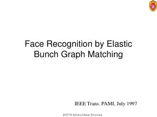
Face Recognition by Elastic Bunch Graph Matching IEEE Trans. PAMI, July 1997
Gabor Transform • Gabor Function Daugman, IEEE Trans. ASSP July 1988 (C) 2005 by Yu Hen Hu
Gabor Wavelet Transform An implementation of Gabor transform Gaussian envelop width = 2 Last term in complex sinusoids removes DC in the kernel 5 level spatial frequency from 4 to 16 pixels in an 128 x 128 image, 8 orientations Daugman, IEEE Trans. ASSP July 1988 (C) 2005 by Yu Hen Hu
Jet a set of 40 (5 spatial frequency, 8 orientations) complex Gabor wavelet coefficients for one image point. J = [a1, a2, …, a40] Similarity between jets: d is the displacement of pixels: needs to be estimated. kj: spatial wave vector Fig. 1. Similarities Sa(J,J’) (dashed line) and S(J,J’) (solid line) with J’ taken from the left eye of a face, and J taken from pixel positions of the same horizontal line. The dotted line shows the estimated displacement d (divided by eight to fit the ordinate range). The right eye is 24 pixels away from the left eye, generating a local maximum for both similarity functions and zero displacement close to dx = -24. (C) 2005 by Yu Hen Hu
Facial fiducial points Pupil, tip of mouth, etc. Face graph Nodes at fiducial pts. Un-directed graph Object-adaptive The structure of graph is the same for each face Fitting a face image to a face graph is done automatically Some nodes may be undefined due to occlusion. Hence, association of nodes of different face graphs may need to be done manually. Bunch A set of Jets all asso with the same fiducial pt. e.g. an eye Jet may consists of different types of eyes: open, closed, male, female, etc. Face bunch graph (FBG): Same as a face graph, except each node consists of a jet bunch rather than a jet Face Graph (C) 2005 by Yu Hen Hu
Face Bunch Graph • Has the same structure as individual face graph • Each node labeled with a bunch of jets • Each edge labeled with average distance between corresponding nodes in face samples • Given a new face, an elastic bunch graph matching (EBGM) method selects the best fitting jets (local experts) from the bunch dedicated to each node in the face bunch graph. (C) 2005 by Yu Hen Hu
Graph similarity measure : weighting factor Initially, manually generate a few FGs to create a FBG Heuristic algorithm to find the image graph that maximizes the similarity: Coarse scan of image using jets to detect face Varying sizes and aspect ratio of FBG to adapt to right format of face. Finally, all nodes are moved locally to maximize SB. Elastic Bunch Graph Matching (C) 2005 by Yu Hen Hu
Results (C) 2005 by Yu Hen Hu