Multiple Regression
Explore how multiple regression analysis considers several variables to explain outcomes, including control and spurious variables, significance testing, model comparison, adjusted R-square, and hypothesis testing.

Multiple Regression
E N D
Presentation Transcript
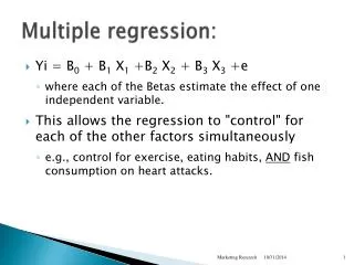
Multiple Regression • Usually several variables influence the dependent variable • Example: income is influenced by years of education and gender • Even if it turns out that we only need one independent variable to explain the model well, it is still good to test it to see if it is really true or whether a competing variable could explain the outcome better.
Mathematical Example • Y= c + aEDU + bSEX + e • What does it mean if years of education has a coefficient of 1000 • What does it mean if gender has a coefficient of 5000? • Y= 100 + a(1000) + b(5000) • Which variable explains income better? • Dummy variables = 0 or 1
Control variables • We want to control whether our variable really is explaining the result or whether some other underlying variable is really at work • Example: we might want to control if the labor market really discriminates against women who have the same jobs as men or whether the problem is that women choose different types of jobs • So we can add “working in the private sectors” as a control variable, since women are more likely to work in the private sector • If gender is still significant then it means that even women, who work in the private sector receive lower salaries than men • If gender is no longer significant it means that the real problem is that either women choose to work in the public sector (but why do they choose this?) • or that women cannot get jobs as easily in the private sector (again the question is why?)
Spurious Variables • A variable is spurious if it seems to predict an outcome, but actually something else is behind it. • In a bivariate regression we have no way of testing for this. • But in a multiple regression, we can see if the variable is still significant once we add a control variable. • In the above example: we might find in a bivariate regression that GENDER is a significant predictor of welfare attitudes, but if it is no longer significant after controlling for WORKING IN THE PRIVATE SECTOR, then it was a spurious (that is misleading) relationship.
Comparing Models • R-square= the amount of variance that a model explains • The higher the r-square the better • How high can R-square be? • Also we want all the variables to be statistically significant at the 5% level.
Adjusted R-square • But if we have 1,000 variables it will normally explain more variance than if we have one. What is the problem? • We want models to be as “parsimonious” as possible. • Adjusted r-square takes into account also the number of variables • That is, it adjusts the r-square downwards to take into account that more variables were added.
Significance • Also we want all the variables to be statistically significant at the 5% level. • That is, t ≥ 1.96 • One variable that was significant in the bivariate regression might become insignificant when controlling for another variable • We also want the entire model to be significant the F-test (this will be discussed at the lab).
Testing Hypotheses • It might be that one author claims that 3 independent variables can explain an outcome. Then you conduct multiple regression and show that with your data only one of these variables is significant. Then you have falsified this previous author’s hypothesis. • You can be satisfied with this falsification or you can go on and try to create a better model. • Often there are several competing theories, so you can test the competing theories by including independent variables from these theories in the regression and see which are significant. • For example, some authors have claimed that CLASS is important in determining socioeconomic attitudes in the Czech Republic. Others have claimed that during the transition, people are not sure what class they belong to, which leads to the hypothesis that INCOME should be more important, since people are more likely to be sure of their income than class. Another hypothesis has been that better educated people are more likely to support the economic reforms, because they can better understand their complexity and thus, understand and believe they should expect cutbacks in welfare support in return for long-term economic growth. So one could – and I DID – take these three variables (CLASS, EDUCATION and INCOME) and use them as independent variables to see which could explain welfare attitudes the best in the Czech Republic.
Answer • Which model has the highest explained variance (R-square)? • What is the problem with Model 1? • If we compare model 2 and model 3, which model explains the greatest amount of variance (R-square)? • Should we choose model 2 then?
Problem of Multicollinearity • Multi = several, more than one • Co = together (cooperate = operate together) • Linear = lines • So it means that several lines have the same slope • In other words, to variables are both measuring the same thing • Example: Gender and Sex
Possible Collinearity in the ISSP • (70) R: Education I: years of schooling and (71) R: Education II-highest education level and (76) Country specific education: Czech Republic • (119) R: Earnings: Czech Republic and (152) Family income: Czech Republic • But it could be less obvious, like (218) R: Religious denomination and (220) R: Attendance of religious services. For example, perhaps among Catholics, only those who attend Church often consider themselves to be Catholics, but most Jews attend services very rarely but still consider themselves to be Jews.
Avoiding Collinearity • The obvious cases we avoid from the beginning. • For example, if I am interested in the influence of Catholicism, then I combine the two variables religious denomination and Church attendence. • First, I make a new variable CATHOLIC and recode demonination so that Catholic = 1 and non-Catholic =0. • Then I create a new variable (CATHDEGR) by multiplying CATHOLIC x Church Attendence, so that regardless of how much one attends services, if they are not Catholic, their score will be 0 • This was especially important for me to do when studying Poland, because almost everyone is Catholic ,so there would be no variation on the variable CATHOLIC but their would be for a new variable DEGREE OF CATHOLICISM
Testing for Collinearity • VIF (Variance Inflation Factor) • If under 10 it is OK • Tolerance statatistic (1/VIF) • Values below 0 .1 indicate serious problems, under 0.2 is cause for concern
Homoscedasticity • At all levels of the independent (i.e. predictor) variables, normally we want the errors to be similarly disributed (homoscedasticity) • It is possible to plot the errors to see if this is true • BUT actually there could be good reasons for the variance to be different at different levels, so it need not be a problem. • Example: in the USA blacks are more likely to vote for Democrats than whiltes. • But whites are more likely to have a higher variance, as whites are rather equally distributed in their voting, while around 90% of blacks vote for Democrats. • In something called ”Maximum Likliehood” models we can actually predict this variance, so it need not be a problem. • BUT you cannot do this with SPSS and it is rather complicated. • So I think you do not have to worry about ”heteroscedasticity”.
Solution? Lay down your statistics textbook Don’t worry BE HAPPY!

