
Adaptive Virtual Queue
E N D
Presentation Transcript
Adaptive Virtual Queue Yang Richard Yang 10/31/2001
Review: Rate Allocation • Rate allocation formulation [Kelly ‘97]
Rate Allocation: Primal-Dual [LL00] • Define • Then the dual problem is to solve xi User i chooses xi such that
Rate Allocation • Recall: • The derivative of D(p) is:
End Hosts and the Network pj(t) xi(t) To control the value of p, the routers observe congestion measures and adjust p Example congestion measure pj(t) • queue length • queueing delay • arrival rate • delay jitter • others Example adaptation algorithms • TCP/Reno (loss) • TCP/SACK (loss) • TCP/Vegas (queueing delay) • TCP-Friendly congestion (loss)
Three Perspectives • Efficiency and fairness • Stability and robustness • Reality
Active Queue Management (AQM) • Objective • generate signal p to users • control queue size • improve utilization • influence loss rate • Issues • how to measure congestion? • queue length at a link • arrival rate at a link • how about combine them?? • how to map from congestion measure to marking (dropping) probability? • why do we need the mapping? • generally, the higher the congestion measure, the higher the mark rate
marking 1 Avg queue RED (Floyd & Jacobson 1993) • Congestion measure: average queue length qj(t+1) = [qj(t) + xj(t) - cj]+ • Mapping: p-linear probability function • Feedback: dropping or ECN marking • Performance • de-synchronization works well • extremely sensitive to parameter setting • fail to prevent buffer overflow as #sources increases
REM (Athuraliya & Low 2000) • Congestion measure: price uj(t+1) = [uj(t) + g(aj (qj(t)-qref)+ xj(t) - cj )]+ • Mapping: exponential probability function • Feedback: dropping or ECN marking
Adaptive Virtual Queue (AVQ) • Based on GKVQ [Gibbens and Kelly ‘99] • Measure congestion by arrival rate At each packet arrival If (VQ+b > B) Mark or drop packet in real queueElseEndif
AVQ System Model queue dynamics
How to Check Whether a System is Stable? • Example 1: • Example 2:
Laplace Transform • Some simple rules • Check the stability of Example 1 characteristic equation
Characteristic Equation where
Performance: Queue Length and VQ Queue length Virtual capacity
Experiment 2: FTP Only Loss Queue length
Experiment 5: Dropping Loss Queue length
Variant: ARED (Feng, Kandlur, Saha, Shin 1999) • Motivation: RED extremely sensitive to #sources • Idea: adapt maxp to load • If avg. queue < minth, decrease maxp • If avg. queue > maxth, increase maxp • No per-flow information needed
Variant: FRED (Lin & Morris 1997) • Motivation: marking packets in proportion to flow rate is unfair (e.g., adaptive vs. unadaptive flows) • Idea • a flow can buffer up to minq packets without being marked • a flow that frequently buffers more than maxq packets gets penalized • all flows with backlogs in between are marked according to RED • no flow can buffer more than avgcq packets persistently • Need per-active-flow accounting
Variant: SRED (Ott, Lakshman & Wong 1999) • Motivation: wild oscillation of queue in RED when load changes • Idea: • estimate number N of active flows • an arrival packet is compared with a randomly chosen active flows • N ~ prob(Hit)-1 • cwnd~p-1/2 and Np-1/2 = Q0implies p = (N/Q0)2 • marking prob = m(q) min(1, p) • No per-flow information needed
Variant: BLUE (Feng, Kandlur, Saha, Shin 1999) • Motivation: wild oscillation of RED leads to cyclic overflow & underutilization • Algorithm • on buffer overflow, increment marking prob • on link idle, decrement marking prob
1 1 1 1 Variant: SFB • Motivation: protection against nonadaptive flows • Algorithm • L hash functions map a packet to L bins (out of NxL ) • marking probability associated with each bin is • Incremented if bin occupancy exceeds threshold • Decremented if bin occupancy is 0 • packets marked with min {p1, …, pL} h1 h2 hL-1 hL nonadaptive adaptive
Variant: SFB • Idea • a nonadaptive flow drives marking prob to 1 at allL bins it is mapped to • an adaptive flow may share some of its L bins with nonadaptive flows • nonadaptive flows can be identified and penalized