Download

1 / 84
920 likes | 1.17k Vues
SEM and Longitudinal Data Latent Growth Models. UTD 07.04.2006. Why Growth models?. Aren‘t autoregressive and cross-lagged models enough to test change and relationships over time? 1) In autoregressive models we can see stability over time but not type of development.

E N D
SEM and Longitudinal DataLatent Growth Models UTD 07.04.2006
Why Growth models? • Aren‘t autoregressive and cross-lagged models enough to test change and relationships over time? • 1) In autoregressive models we can see stability over time but not type of development. • We might have a stability of 1 – that is the relative placement of people is unchanged, and still everyone increases (or decreases).
Number of cigarettes smoked after meal as a function of the day of the course
Stability is 1 in an autoregressive model. Higher ones remain higher, and lower ones remain lower. • However, there is a development. They all increase the number of cigarettes smoked. We cannot see it in the autoregressive model. • We need a developmental model, which takes into account this development, but- also the differences in development across individuals.
In the example, each individual had an intercept and a slope. • Person1 had a slope 1, and an intercept 1 • Person2 had a slope 1, and an intercept 2 • Person3 had a slope 1, and an intercept 3 • The mean of their slope is 1 • The mean of their intercept is 2 • The developmental model should take this individual information into account • Still, the model should allow us to study development at the group level
The Latent Growth Curve Model • These criteria are met by the growth curve model. Meredith and Tissak (1990) belonged to the first to develop the growth model mathematically. • The model uses an SEM methodology • The results are meaningful when there is time gap between the measurements, and not just repeated measures • How long the time gap is between the time points- is also meaningful • The number of time points and the spacing between time points across individuals should be the same
The latent factors in the growth model are interpreted as common factors representing individual differences over time. • Remark: Latent growth model was developped from ANOVA, and expanded over time. • Basically, with two time points we can have only a linear process of change. However, for deductive purpose, we will start with modeling a growth model for two time points, and then expand it to more points in time.
Intercept: The intercept represents the common or mean intercept for all individuals, since it has a factor loading of 1 to all the time points. In the previous example it will have a mean 2. It is the point where the common line for all individuals crosses the y axis. • It presents information in the sample about the mean and variance of the collection of intercepts that characterize each individual‘s growth curve.
Slope: It represents the slope of the sample. In this case it is the straight line determined by the two repeated measures. It also has a mean and a variance, that can be estimated from the data. • Slope and intercept are allowed to covary. • In this example with two time points, in order to get the model identified, the coefficients from the slope to the two measures have to be fixed. For ease of interpretation of the time scale, the first coefficient is fixed to zero. • With a careful choice of factor loadings, the model parameters have familiar straightforward interpretations.
Exercise:is the model identified? How many df? How many parameters are to be estimated? • In this example: • The intercept factor represents initial status • The slope factor represents the difference scores anomia2-anomia1 since: • Anomia1=1*Intercept + 0*Slope + e1 • Anomia2=1*Intercept + 1*Slope + e2 • If errors are the same then • Anomia2 – Anomia1 = Slope
This model is just identified (if we set the measurement errors to zero). By expanding the model to include error variances, the model parameters can be corrected for measurement error, and this can be done when we have three measurement time points or more. • Three or more time points provide an opportunity to check non linear trajectories. • For those interested, Duncan et al. Shows the technical details for this model on p. 15-19.
Representing the shape of growth • With three points in time, the factor loadings carry information about the shape of growth over time. • In this example we specify a linear model. We have reasons to believe that anomia is increasing as a linear process, and this way we can test it. • If we are not sure, we can test a model where the third factor loading is free
Parallel stability Linear stability level level time time Strict stability Monotone stability level level time
Sometimes there are reasons to believe that the process is not linear. For example, a process might take a quadratic form. • In this case, one can model a three-factor polynomial LGM • Anomia=intercept +slope1*t+slope2*t2 • However, this is more rare in sociology and political sciences. It might be reasonable in contexts such as learning, tobacco reduction etc.
Summary1 • In all the examples shown we use LGM when we believe that the process at hand is a function of time. • What is the meaning of the covariance between slope and intercept? Intercept represents the initial stage, and slope the change. A negative covariance suggests that people with a lower initial status, change more and people with a higher initial status change less. • For positive covariances: people with a higher initial status change more, and people with a lower initial status change less.
Summary 2 • There is no direct test for cross lagged effects. • The means of the latent slope and the latent intercept represent the developmental process over time for the whole group; their variance represents the individual variability of each subject around the group parameters.
Single-indicator model vs. multiple-indicator model • Instead of using a single-scale score to measure at each time point authoritarianism or anomie for example, we could use latent factors to estimate these constructs, and could therefore be purged from measurement error.
In a 2nd order LGM • The same 1st order variable is chosen as the scale indicator for each first-order factor. Corresponding variables whose loadings are free have those loadings constrained to be equal across time. This ensures a comparable definition of the construct over time (referred to as „stationarity“, Hancock, Kuo & Lawrence 2001, Tisak and Meredith 1990).
Measurement Invariance: Equal factor loadings across groups Group A Group B dB11 Item a dA11 lB11=1 Item a lA11=1 fB11 k B1 fA11 k A1 Bt1 At1 lB21 lA21 dB22 dA22 Item b Item b lB31 lA31 Item c Item c dB33 dA33 fB21 fA21 dB44 dA44 Item d Item d lB42=1 lA42=1 Bt2 At2 lB52 lA52 Item e Item e dB55 dA55 lB62 lA62 fB22 k B2 fA22 k A2 dB66 dA66 Item f Item f
Steps in testing for Measurement Invariance between groups and/or over time • Configural Invariance • Metric Invariance • Scalar Invariance • Invariance of Factor Variances • Invariance of Factor Covariances • Invariance of latent Means • Invariance of Unique Variances
Steps in testing for Measurement Invariance • Configural Invariance • Metric Invariance • Equal factor loadings • Same scale units in both groups/time points • Presumption for the comparison of latent means • Scalar Invariance • Invariance of Factor Variances • Invariance of Factor Covariances • Invariance of latent Means • Invariance of Unique Variances
Full vs. Partial Invariance • Concept of ‘partial invariance’ introduced by Byrne, Shavelson & Muthén (1989) • Procedure • Constrain complete matrix • Use modification indices to find non-invariant parameters and then relax the constraint • Compare with the unrestricted model • Steenkamp & Baumgartner (1998): Two indicators with invariant loadings and intercepts are sufficient for mean comparisons • One of them can be the marker + one further invariant item
Autocorrelation • As in the autoregressive model, we believe that measurement errors of repeated measures are related to one another. Therefore, we correlate them (Hancock, Kuo & Lawrence 2001, Loehlin 1998).
Intercepts • In a 2nd order factor LGM, intercepts for corresponding 1st order variables at different time points are constrained to be equal, reflecting the fact that change over time in a given variable should start at the same initial point.
MIMIC and LGM, time-invariant covariates in the latent growth modeling • Sometimes a model in which longitudinal development is predicted by an intercept and growth curve is too restrictive. Such a model is called unconditional. In such a case we may try to predict the latent slope and intercept by background variables (for example demographic variables), which are time invariant. This would be called a conditional model.
Another complication: the intercept and slope may be not only conditioned on some other variables, they could also cause them. For example, the intercept of anomia could be a cause of a variable named satisfaction in life.
Analyzing growth in multiple populations • Sometimes our data contains information on several populations: males and females, different age cohorts, people from former east and west Germany, voters of right and left wing parties, ethnicities, treatment and control groups etc. • The SEM methodology to analyze multiple groups can be applied also here. We can compare the means of the slope and intercept latent variables as well as growth parameters, equality of covariance between slope and intercept etc.
The coding of time (Biesanz, Deeb-Sossa, Papadakis, Bollen and Curran, 2004) • Misinterpretation regarding the relationships among growth parameters (intercepts and slopes) appear frequently. Therefore it is important to pay attention to the coding of time • Covariance between intercept and slope, and variance of the intercept and slope are directly determined by the choice of coding • When the coefficient between slope and the first time point is set to zero, the covariance and variances are related to the first time point. For example, a negative covariance between the slope and intercept indicates that at the first (0) time point people with a lower starting point change more quickly. It is not necessarily true for later time points.
If we are interested at the relation between the intercept and the slope at a later time point, for example the second one, we have to fix at this point the coefficient from the slope to zero. The first coefficient will change from 0 to -1, and the third coefficient will change from 2 to 1. • It is useful to code the coefficients from the slope according to the time interval on a yearly basis, if we believe in a linear process.
Example: if we have data collected in January, then in July, and then again in July in the following year, a possible coding of the coefficients from the slopes to the measurements could be: • 0, 0.5 (since the measurement took place half a year later) and 1.5. • Exercise: If we are interested in the relations between the slope and the intercept at the second time point, how could we code the coefficients?
Answer: -0.5, 0 and 1. • Using a yearly basis, we keep the interpretation simple. • If we have a quadratic model, the interpretation of the highest order coefficient (for example its variance) does not change with different codings and placement of time origins. But the interpretation of lower order terms (intercept and linear slope) does. • The choice of where to place the origin of time has to be substantially driven. This choice determines that point in time at which individual differences will be examined for the lower order coefficients.
Level of anomia 2.0 1.5 1.0 time
Coding and Mimic • The meaning of the variance of the intercept and the slope changes in Mimic models. If the intercept is explained (conditioned) by age for example, the residual variance of the intercept indicates the variability across individuals in the starting point not accounted for by age. • This should be taken into account when we interpret our results.
The bivariate latent trajectories (growth curve) analysis • We can extend the univariate latent trajectory model to consider change in two or more variables over time. • The bivariate trajectory model is simply the simultaneous estimation of two univariate latent trajectory models. • The relation between the random intercepts and slopes is evaluated for each series. Then it is possible to determine whether development in one behavior covaries with other behaviors.
So far we could demonstrate LGM which allow multiple measures, multiple occasions and multiple behaviors simultanuously over time. • We could estimate the extent of covariation in the development of pairs of behaviors. • We can go one level higher, and extend the test of dynamic associations of behaviors by describing growth factors in terms of common higher order constructs.
Factor-of-curves LGM • To test whether a higher order factor could describe the relations among the growth factors of different processes, the models can be parameterized as a factor of curves LGM. • The covariances among the factors are hypothesized to be explained by the higher order factors (McArdle 1988). • The method is useful in determining the extent to which pairs of behaviors covary over time. • Rarely used. The test if the approach is better can be done by comparing the fit measures of alternative models.
Factor-of-curves LGM d2 d1 d3 d4
Missing values and LGM • As in AR models, missing data constitute a problem in LGM. Also here we distinguish between 3 kinds of MD: MCAR, MAR and MNAR. • The diagnosis and solutions discussed in the AR apply also for LGM models.
Estimating Means and Getting the model identified • As Sörbom (1974) has shown, in order to estimate the means, we must introduce some further restrictions: • 1) setting the mean of the latent variable in one group-the reference group- to zero. The estimation of the mean of the latent variable in the other group is then the mean difference with respect to the reference group. In the growth model, one could alternatively set all intercepts of the constructs in both groups to zero and intercept of one indicator per construct to zero (constraining the second to be equal across time points), and then compare the means of the latents mean and intercepts in both groups. • 2) in case of a one group analysis: setting the measurement models invariant across time, since it makes no sense to compare the means of constructs having a different measurement model over time. At least one intercept (of an indicator) per construct has to be set equal across time.