System Dynamics
In this class, we shall introduce a new Dymola library designed to help us with modeling population dynamics and similar problems that are described as pure mass flows .


System Dynamics
E N D
Presentation Transcript
In this class, we shall introduce a new Dymola library designed to help us with modeling population dynamics and similar problems that are described as pure mass flows. The system dynamics methodology had been introduced in the late sixties by J.W.Forrester as a tool for organizing partial knowledge about models of systems from soft-sciences, such as biology, bio-medicine, and macro-economy. System Dynamics
From bond graphs to system dynamics Exponential growth Levels and rates Gilpin model Laundry list System dynamics modeling recipe Larch bud moth Influenza Table of Contents
Remember how we have been modeling convective flows (mass flows) using bond graphs. . . . . . . From Bond Graphs to System Dynamics I
If we weren’t interested, where the energy came from, we could leave the pumps out, and replace them by flow sources. e1 = e(t) f1 = f(t) der(q) = f1 – f2 e = C(q) f2 = f(t) e2 = e(t) From Bond Graphs to System Dynamics II
If we furthermore aren’t interested in the efforts at all, the effort equations can be left out, and all the bonds become activated, i.e., turn into signal flows. e1 = e(t) f1 = f(t) der(q) = f1 – f2 e = C(q) f2 = f(t) e2 = e(t) From Bond Graphs to System Dynamics III
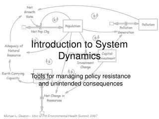
Forrester introduced a graphical representation tailored to exactly this situation. From Bond Graphs to System Dynamics IV
Let us start by implementing the simple exponential growth model that had been introduced two classes ago: · P = BR – DR BR = kBR· P DR = kDR· P Source and sink elements are provided for optical purposes only, because the systems dynamics modelers are used to them. However, these models do not contain any equations. Exponential Growth Model
Levels represent the state variables of the system dynamics modeling methodology. This is an InPort drawn the wrong way for optical reasons. An explanation follows shortly. Levels
Rates represent the state derivatives of the system dynamics modeling methodology. Rates I
For convenience, rates with multiple additive inputs are also provided. Notice that this is an OutPort that was drawn in reverse for optical reasons. Whereas mass can be envisaged to flow from the source to the level at a rate controlled by the rate valve, the flow of information, however, is from the rate to the source. Rates II
Also available are rate gauges with built-in limiters, e.g. valves that let flow pass in one direction only. RatesIII
Also available are levels with overflow protection and with protection against pumping from an already empty storage. Levels II A Boolean variable that is set false when the tank is full. Another Boolean variable that is set false when the tank is empty.
We now have everything that we need to create a system dynamics version of the Gilpin model. The Gilpin Model I This model can be compiled.
What have we gained by representing the Gilpin model in the system dynamics formalism? System dynamics is not particularly useful for implementing an already fully developed model, such as the Gilpin model. The Gilpin Model IV Absolutely nothing! Systems dynamics has been invented as a tool for graphically capturing partial knowledge about a poorly understood system, generating a model that can be successively augmented, as new knowledge becomes available.
Levels Rates Inflows Outflows Population Birth Rate Death Rate Money Income Expenses Frustration Stress Affection Love Affection Frustration Tumor Cells Infection Treatment Inventory on Stock Shipments Sales Knowledge Learning Forgetting • Population • Material Standard of Living • Food Quality • Food Quantity • Education • Contraceptives • Religious Beliefs Birth Rate: The Laundry List • System dynamics, just like any other decent modeling methodology, always starts out with the set of variables to be used in the model, especially the levels and the rates. For each of the rates, a list of the most influential variables is created. This is called a laundry list.
System Dynamics Modeling Recipe • We always start out by choosing the levels to be included in the model. These must be quantities that can be accumulated. • For each level, we define one or several additive inflows and one or several additive outflows. These are the rates. • For each rate, we define a laundry list comprised of the set of most influential factors. • For each of these factors, equations are generated that relate these factors back to the levels, the rates, and other factors. These equations are created by using as much physical insight as possible. Algebraic loops are to be avoided.
The Larch Bud Moth Model I • We shall now attempt to come up with a better model for describing the population dynamics of the larch bud moth making use of the systems dynamics modeling methodology. • We stipulate that the insect/tree interaction is the dominant influencing factor regulating the population dynamics of the larch bud moth. We assume that the influence of the parasites is of second order small, and can be neglected. • We shall try to come up with a model based primarily on physical insight. • Curve fitting shall be used, but limited to local measurable properties only.
The Larch Bud Moth Model II • The insects breed only once per year. They lay their eggs onto the branches of the larch trees in August. The eggs then remain in a state of extended embryonic diapause until the following spring. • Hence it makes sense to use a discrete-time model, i.e., describe the population dynamics of the larch bud moth by a set of difference equations. • To this end, a discrete level model is being offered as part of Dymola’s SystemDynamics library.
The when-clause is executed for the first time at time=h, then once every h time units. Discrete Levels • Discrete levels are another form of state variables for the system dynamics modeling methodology.
The Larch Bud Moth Model III • There are two discrete state variables: the number of eggs, and the raw fiber, which the insect larvae use as their food. Since both the eggs and the needle mass are being replaced every year, the old eggs and old fibers simply all go away. Thus, the outflows are equal to the levels.
During the fall, the eggs are preyed upon by several species of Acarina and Dermaptera. During the winter, the eggs are parasitized by a species of Trichogramma. The surviving eggs are ready for hatching in June. The overall effects of winter mortality can be summarized as a simple constant. The Larch Bud Moth Model IV Small_larvae = (1.0 – winter_mortality) · Eggs winter_mortality = 57.28%
Gain factors are modeled as follows: Gain Factors
Whether or not the small larvae survive, depends heavily on luck or mishap. For example, if the branch on which the eggs have been laid dies during the winter, the young larvae have no food. This is called the incoincidence factor. However, the incoincidence factor is not constant. It depends heavily on the raw fiber contents of the biomass of the tree. The Larch Bud Moth Model V Large_larvae = (1.0 – incoincidence) · Small_larvae
A linear regression model was used to determine the incoincidence factor from measurements: Linear Regression incoincidence = 0.05112 · rawfiber – 0.17932
The Larch Bud Moth Model VI • Hence we can model the population of large larvae using two “linear regression” models in series, followed by a two-input product model: incoincidence = 0.05112 · rawfiber – 0.17932 coincidence = (-1.0) · incoincidence + 1.0 Large_larvae = coincidence · Small_larvae
The Larch Bud Moth Model VII • In similar ways, we can model the entire egg life cycle: • The animal population is further decimated, either because the large larvae don’t have enough food (starvation), or because they were sick already before (physiological weakening). Small_larvae = (1.0 – winter_mortality) · Eggs Large_larvae = (1.0 – incoincidence) · Small_larvae Insects = (1.0 – starvation) · (1.0 – weakening) · Large_larvae Females = sex_ratio · Insects New_eggs = fecundity · Females
The Larch Bud Moth Model VIII • Notice that we essentially created a physical model of the entire egg life cycle. • Curve fitting is only used locally to identify linear regression models of measurable physical quantities. • The sex ratio is constant, whereas starvation depends on food demand and tree foliage (food supply): incoincidence = 0.05112 · rawfiber – 0.17932 weakening = 0.124017 · rawfiber – 1.435284 fecundity = -18.475457· rawfiber + 356.72636 sex_ratio = 0.44 starvation = f1 (foliage, food_demand) food_demand = 0.005472 · Large_larvae
In similar ways, we can model the life cycle of the trees: where: The Larch Bud Moth Model IX New_rawfiber = recruitment · rawfiber recruitment = f2 (defoliation, rawfiber) defoliation = f3 (foliage, food_demand, starvation) foliage = specific_foliage · nbr_trees specific_foliage = -2.25933· rawfiber + 67.38939 nbr_trees = 511147
We started out by deciding on the formalism itself, i.e., we decided that we were going to use discrete rather than continuous levels. We then identified the number of levels, i.e., the number of quantities that can be independently accumulated. In our case, we decided on using the eggs and the raw fiber as the two state variables. We then identified life cycles for the two levels. We limited curve fitting to identifying locally verifiable relationships between variables, which in our case turned out to be linear regression models. This provided us with an almost complete model. There are only three laundry lists: f1, f2, and f3 that require further analysis. The Larch Bud Moth Model XI
The SystemDynamics library offers three partial blocks for capturing functional relationships, one for functions with a single input, one for functions with two inputs, and one for functions with three inputs. Functional Relationships
This block was used to create a model for the starvation: The Larch Bud Moth Model XII
The equation window of the main model looks as follows: Notice that no global curve fitting was ever applied to this model. The Larch Bud Moth Model XIV
We are now ready to compile and simulate the model. The Larch Bud Moth Model XV
The model reproduces the observed limit cycle behavior of the larch bud moth population beautifully, both in terms of amplitude and frequency. The Larch Bud Moth Model XVI Since no global curve fitting was applied to the model, this is an indication that the important relationships were modeled correctly.
Let us create yet one more model today, describing the spreading of an influenza epidemic in a community of 10,000 souls. Since influenza can be contracted at any time, we shall use continuous levels for this model. People, once infected with this particular variant of the disease, take four weeks before they come down with any symptoms. This is called the incubation period. Yet, they are already contagious during that period. Once they are sick, they remain sick for two weeks. Once they have recovered from the disease, they are immune to this particular stem for 26 weeks. Thereafter, they may contract the disease anew. The Influenza Model I
Let us now choose our level variables. We can identify four types of people: We shall use these four variables as our levels. Clearly, there are only three state variables, since the sum of the four is always 10,000, i.e., we can always compute the fourth from the other three, but as long as we don’t insist that we must choose our initial conditions independently, this doesn’t cause any problem. The Influenza Model II • Non-infected people. • Infected healthy people. • Sick people. • Immune people.
The four level variables are placed in a loop. They are fed by four rate variables: We shall use these four variables as our rates. The Influenza Model III • Contraction rate. • Incubation rate. • Recovery rate. • Re-activation rate.
The contraction rate can be computed as the product of the percentage of contagious population multiplied with the number of contacts per week multiplied with the probability of contracting the disease on a single contact. The incubation rate can be computed as the quotient of the infected population and the time to breakdown. The recovery rate can be computed as the quotient of the sick population and the duration of the symptoms. The re-activation rate can be computed as the quotient of the immune population and the immune period. The Influenza Model IV
We want to take into account that the numbers in each level are supposed to be integers. By default, theinteger functionwill schedule events inDymola. As this is not useful here, we use thenoEvent clauseto prevent these unnecessary event iterations from happening. The Influenza Model VI
One additional problem concerning the contraction rate needs to be taken care of. It could theoretically happen that the model tries to infect more people than the total uninfected population. This must be prevented. The Influenza Model VII
The equation window of the main model looks as follows: At time = 8 weeks, we introduce one single influenza patient into the general population of our community. The Influenza Model VIII
The model can now be compiled. The Influenza Model IX
Simulation results: Within only 6 weeks, almost the entire population of the community has been infected with the disease. The epidemiology of the disease is just as bad as that of the chain letter! The Influenza Model X
We have now improved our skills for developing soft-science models in an organized fashion that stays as close to the underlying physics as can be done. System dynamics was introduced as a methodology that allows us to formulate and capture partial knowledge about any soft-science application, knowledge that can be refined as more information becomes available. Systems dynamics is the most widely used modeling methodology in all of soft sciences. Tens of thousands of scientists have embraced and used this methodology in their modeling endeavors. Conclusions
Cellier, F.E. (1991), Continuous System Modeling, Springer-Verlag, New York, Chapter 11. Fischlin, A. and W. Baltensweiler (1979), “Systems analysis of the larch bud moth system, Part 1: The larch – larch bud moth relationship,” Mitteilungen der Schweiz. Entomologischen Gesellschaft, 52, pp. 273-289. Cellier, F.E. (2007), The Dymola System Dynamics Library, Version 2.0. References