Systematics in the Pierre Auger Observatory
410 likes | 611 Vues
Systematics in the Pierre Auger Observatory. Bruce Dawson University of Adelaide for the Pierre Auger Observatory Collaboration. Introduction. Fluorescence - a technique with great rewards, but a lot of work required!

Systematics in the Pierre Auger Observatory
E N D
Presentation Transcript
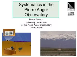
Systematics in the Pierre Auger Observatory Bruce Dawson University of Adelaidefor the Pierre Auger Observatory Collaboration
Introduction • Fluorescence - a technique with great rewards, but a lot of work required! • Will concentrate on energy measurement (e.g. composition has an additional set of systematics) • All good experiments build in CROSS-CHECKS, Auger no exception. Clearly, most important cross-check is the Hybrid nature of Auger, but many others.
The Observatory • Mendoza Province, Argentina • 3000 km2, 875 g cm-2 • 1600 water Cherenkov detectors 1.5 km grid • 4 fluorescence eyes -total of 24 telescopes each with 30o x 30o FOV 65 km
Simulated Hybrid Aperture “Stereo” Efficiency Hybrid TriggerEfficiency
Hybrid Reconstruction Quality Statistical errors only! • 68% error bounds given • detector is optimized for 1019eV, but good Hybrid reconstruction quality at lower energy statisticalerrors only zenith angles < 60O
Steps to good energy reconstruction • Geometry • Calibration: atmosphere and optical • Analysis • Light collection • Cherenkov subtraction • Fitting function • Missing energy • Fluorescence yield
Geometry Reconstruction • eye determines plane containing EAS axis and eye • plane normal vector known to an accuracy of ~ 0.2o • to extract Rp andy,eye needs to measure angular velocity w and its time derivative dw/dt • but difficult to get dw/dt, leads to degeneracy in (Rp,y) • degeneracy broken with measurement of shower front arrival time at one or more points on the ground • eg at SD water tank positions
Geometry Reconstruction Single FD only Hybrid median Rp error = 350mstrong dependence on angular “Track Length” medianRp error = 20 m • Simulations at 1019eV • Reconstruct impact parameter Rp. Dramatic improvement with Hybrid reconstruction (Will check with stereo events)
Atmosphere Systematics • light transmission corrections(Rayleigh and aerosol scattering)AIM: know corrections to better than 10% • air density profile with height(mapping height to depth; Rayleigh scattering)AIM: know overburden at a given height to better than 15 g/cm2
Distance from pixels to track MC: 1019eV events over full arrayClosest triggering eye
Horizontal attenuation monitors (50km) • Steerable LIDARs - total optical depth • Vertical lasers near centre of array - vertical distribution of aerosols • Cross-checks
Aerosol measurements (John Matthews ICRC 2001)
LIDAR System Tests near Torino System at Los Leones
Some simulations • Simulations: 1000 1019eV showers landing within Auger full array. Generate with fixed aerosol parameters: • horizontal attenuation length (334nm) al = 25 km • scale height of aerosol layer ha = 1.0 km • height of “mixing layer” hm = 0 km • First, reconstruct events with different aerosol assumptions
Dependence on Aerosol Parameters • (generated with al=25km, ha=1.0km, hm=0km) • reconstruct with 19km 1.0km 0kmDE/E = +8%DXmax = +7 g/cm2 • reconstruct with 40km 1.0km 0kmDE/E = -9%DXmax = -9 g/cm2 • reconstruct with 25km 2.0km 0kmDE/E = +10%DXmax = -2 g/cm2 • reconstruct with 25km 1.0km 0.5kmDE/E = +12%DXmax = +8 g/cm2
Atmosphere Density Profile • Density profile of atmosphere determines mapping from height to depth, and Rayleigh scattering • MC generated with vertical overburden 873 g/cm2andone of the US Standard Atmospheres. Will maintain scale height. • reconstruct with vertical overburden900 g/cm2DE/E = +2.2%DXmax = +19 g/cm2 • reconstruct with vertical overburden845 g/cm2DE/E = - 3.3%DXmax = - 19 g/cm2
Radiosonde • Balloon-borne radiosondes are planned to monitor the atmosphere’s density and temperature profile • First flight in August 2002 at Malargue. • A series of flights in the austral spring, summer, winter and autumn will determine the suitability of re-scaled “standard atmospheres”, and variability.
Drum Calibration • 375nm LEDs • NIST calibrated Silicon detector • uniformly illuminates aperture with full range of incoming angles • in future will also use range of colours • absolute calib to 7% now, hope to improve to 5%
Laser shots at 3km - cross check on absolute calibration … and also are checking with piece by piece calibration.
UV-Filter 300-400 nm installed at Los Leones (Malargüe) and taking data 11 m2 mirror camera440 PMTs corrector lens
Hybridevent.Dec 2001- March2002
Light Flux at Camera z=1.9o z=3o optical spot 0.5 deg diam • Aim: to collect all signal without too much noise or multiple scattered light. • Effect of multiple scattered light? Halo? • currently a 10-15% systematic, is being studied
Estimate of Cherenkov contamination Total F(t) photons (equiv 370nm) direct Rayleigh aerosol time (100ns bins) REAL event
Dependence on Cherenkov Yield • MC generated with nominal Cherenkov yield • (easy calculation if you know the density profile of atmosphere and the energy spectrum of electrons) • reconstruct with Cherenkov yield up by 30%DE/E = - 4.8%DXmax = - 9 g/cm2 • reconstruct with Cherenkov yield reduced by 30%DE/E = + 5.3%DXmax = +9 g/cm2 • (These are averages. Clearly, the error for each event depends on its geometry).
Cherenkov correction • clearly depends on more than yield calculation, also… • atmospheric scattering • geometry • important problem that needs study, since all events have some contamination • stereo will be an important aid
PRELIMINARY shower size (arb units)
PRELIMINARY shower size (arb units)
Profile T. Abu-Zayyad et al Astropart. Phys. 16, 1 (2001)
“Missing energy” correction • unavoidable 5% systematic • currently being checked with new CORSIKA Ecal = calorimetric energyE0 = true energy from C.Song et al. Astropart Phys (2000)
Conclusion • can’t provide an error budget now - many of the systematics are under study, and we need real (stereo) data to study many of them • have indicated our goals in terms of two major players - the atmosphere (10%) and optical calibration (5%). These must be obtained early. • cross-checks are vital • then there is the fluorescence yield…