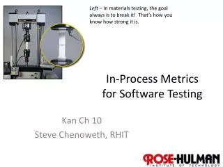
Topics in Metrics for Software Testing

1. Topics in Metrics for Software Testing [Reading assignment: Chapter 20, pp. 314-326]

2. Quantification • One of the characteristics of a maturing discipline is the replacement of art by science. • Early physics was dominated by philosophical discussions with no attempt to quantify things. • Quantification was impossible until the right questions were asked.

3. Quantification (Cont’d) • Computer Science is slowly following the quantification path. • There is skepticism because so much of what we want to quantify it tied to erratic human behavior.

4. Software quantification • Software Engineers are still counting lines of code. • This popular metric is highly inaccurate when used to predict: • costs • resources • schedules

5. Science begins with quantification • Physics needs measurements for time, mass, etc. • Thermodynamics needs measurements for temperature. • The “size” of software is not obvious. • We need an objective measure of software size.

6. Software quantification • Lines of Code (LOC) is not a good measure software size. • In software testing we need a notion of size when comparing two testing strategies. • The number of tests should be normalized to software size, for example: • Strategy A needs 1.4 tests/unit size.

7. Asking the right questions • When can we stop testing? • How many bugs can we expect? • Which testing technique is more effective? • Are we testing hard or smart? • Do we have a strong program or a weak test suite? • Currently, we are unable to answer these questions satisfactorily.

8. Lessons from physics • Measurements lead to Empirical Laws which lead to Physical Laws. • E.g., Kepler’s measurements of planetary movement lead to Newton’s Laws which lead to Modern Laws of physics.

9. Lessons from physics (Cont’d) • The metrics we are about to discuss aim at getting empirical laws that relate program size to: • expected number of bugs • expected number of tests required to find bugs • testing technique effectiveness

10. Metrics taxonomy • Linguistic Metrics: Based on measuring properties of program text without interpreting what the text means. • E.g., LOC. • Structural Metrics: Based on structural relations between the objects in a program. • E.g., number of nodes and links in a control flowgraph.

11. Lines of code (LOC) • LOC is used as a measure of software complexity. • This metric is just as good as source listing weight if we assume consistency w.r.t. paper and font size. • Makes as much sense (or nonsense) to say: • “This is a 2 pound program” • as it is to say: • “This is a 100,000 line program.”

12. Lines of code paradox • Paradox: If you unroll a loop, you reduce the complexity of your software ... • Studies show that there is a linear relationship between LOC and error rates for small programs (i.e., LOC < 100). • The relationship becomes non-linear as programs increases in size.

13. Halstead’s program length

14. Example of program length n = 9 (if, <, =,- (sign), while, if (y < 0) pow = - y; else pow = y; z = 1.0; while (pow != 0) { z = z * x; pow = pow - 1; } if (y < 0) z = 1.0 / z; 1 ! =, *, - (minus), /) n = 7 (y, 0, pow, z, x, 1, 1.0) 2 » H = 9 log 9 + 7 log 7 48 2 2

15. Example of program length for ( j=1; j<N; j++) { last = N - j + 1; for (k=1; k <last; k ++) { if (list[k] > list[k+1]) { temp = list[k]; list[k] = list[k+1]; list[k+1] = temp; } } } n = 9 (for, =, <, + +, -, +, [], >, if) 1 n = 7 (j, 1, N, last, k, list, temp) 2 » H = 9 log 9 + 7 log 7 48 2 2

16. Halstead’s bug prediction

17. How good areHalstead’s metrics? • The validity of the metric has been confirmed experimentally many times, independently, over a wide range of programs and languages. • Lipow compared actual to predicted bug counts to within 8% over a range of program sizes from 300 to 12,000 statements.

18. Structural metrics • Linguistic complexity is ignored. • Attention is focused on control-flow and data-flow complexity. • Structural metrics are based on the properties of flowgraph models of programs.

19. Cyclomatic complexity • McCabe’s Cyclomatic complexity is defined as: M = L - N + 2P • L = number of links in the flowgraph • N = number of nodes in the flowgraph • P = number of disconnected parts of the flowgraph.

20. Property of McCabe’s metric • The complexity of several graphs considered together is equal to the sum of the individual complexities of those graphs.

21. Examples of cyclomatic complexity L=1, N=2, P=1 M=1-2+2=1 L=4, N=4, P=1 M=4-4+2=2 L=2, N=4, P=2 M=2-4+4=2 L=4, N=5, P=1 M=4-5+2=1

22. Cyclomatic complexity heuristics • To compute Cyclomatic complexity of a flowgraph with a single entry and a single exit: • Note: • Count n-way case statements as N binary decisions. • Count looping as a single binary decision.

23. _____ A&B&C _ _ A A ___ _ _ B&C B C Compound conditionals • Each predicate of each compound condition must be counted separately. E.g., A&B&C A&B&C M = 2 A B&C A B&C M = 3 A C A B C M = 4

24. Cyclomatic complexity of programming constructs 2 1. if E then A else B 2. C 1 1. loop A 2. exit when E B 3. end loop 4. C 2 2 3 M = 2 1 M = 2 1. case E of 2. a: A 3. b: B … k. k-1: N l. end case m. L 4 ... K 2 3 1. A B C … 2. Z 1 l 2 m M = 1 M = (2(k-1)+1)-(k+2)+2=K-1

25. Applying cyclomatic complexity to evaluate test plan completeness • Count how many test cases are intended to provide branch coverage. • If the number of test cases < M then one of the following may be true: • You haven’t calculated M correctly. • Coverage isn’t complete. • Coverage is complete but it can be done with more but simpler paths. • It might be possible to simplify the routine.

26. Warning • Use the relationship between M and the number of covering test cases as a guideline not an immutable fact.

27. Nm+kNc Lm+kLc 0 0 Nm Lm+k Nc+2 Lc Lm+kLc-Nm-kNc+2 0 Lm+kLc-Nm-kNc+2 Lm+k-Nm+2 Lc-Nc-2+2=Lc-Nc=Mc Lm+Lc-Nm-Nc+k+2 Main Nodes Main Links Subnodes Sublinks Main M Subroutine M Total M Subroutines & M Embedded Common Part Subroutine for Common Part

28. When is the creation of asubroutine cost effective? • Break Even Point occurs when the total complexities are equal: • The break even point is independent of the main routine’s complexity.

29. Example • If the typical number of calls to a subroutine is 1.1 (k=1.1), the subroutine being called must have a complexity of 11 or greater if the net complexity of the program is to be reduced.

30. Cost effective subroutines (Cont’d)

31. Cost effective subroutines (Cont’d)

32. Relationship plotted as a function Mc • Note that the function does not make sense for values of 0 < k < 1 because Mc < 0! • Therefore we need to mention that k > 1. 1 0 1 k

33. How good is M? • A military software project applied the metric and found that routines with M > 10 (23% of all routines) accounted for 53% of the bugs. • Also, of 276 routines, the ones with M > 10 had 21% more errors per LOC than those with M <= 10. • McCabe advises partitioning routines with M > 10.

34. Pitfalls • if ... then ... else has the same M as a loop! • case statements, which are highly regular structures, have a high M. • Warning: McCabe’s metric should be used as a rule of thumb at best.

35. Rules of thumb based on M • Bugs/LOC increases discontinuously for M > 10 • M is better than LOC in judging life-cycle efforts. • Routines with a high M (say > 40) should be scrutinized. • M establishes a useful lower-bound rule of thumb for the number of test cases required to achieve branch coverage.

36. Software testing process metrics • Bug tracking tools enable the extraction of several useful metrics about the software and the testing process. • Test managers can see if any trends in the data show areas that: • may need more testing • are on track for its scheduled release date • Examples of software testing process metrics: • Average number of bugs per tester per day • Number of bugs found per module • The ratio of Severity 1 bugs to Severity 4 bugs • …

37. Example queries applied to a bug tracking database • What areas of the software have the most bugs? The fewest bugs? • How many resolved bugs are currently assigned to John? • Mary is leaving for vacation soon. How many bugs does she have to fix before she leaves? • Which tester has found the most bugs? • What are the open Priority 1 bugs?

38. Example data plots • Number of bugs versus: • fixed bugs • deferred bugs • duplicate bugs • non-bugs • Number of bugs versus each major functional area of the software: • GUI • documentation • floating-point arithmetic • etc

39. Example data plots (cont’d) • Bugs opened versus date opened over time: • This view can show: • bugs opened each day • cumulative opened bugs • On the same plot we can plot resolved bugs, closed bugs, etc to compare the trends.

40. You now know … • … the importance of quantification • … various software metrics • … various software testing process metrics and views