Decision Procedures for Linear Arithmetic
This presentation, led by Omer Katz, delves into decision procedures for linear arithmetic, highlighting key algorithms and techniques such as DPLL-T for solving SMT problems. It covers fundamental concepts including Gaussian elimination, Fourier-Motzkin elimination, and the Simplex method, addressing their applications and limitations. The discussion also includes preprocessing enhancements and the relationship between linear inequalities and computational feasibility. This complex topic is essential for computer science professionals and researchers exploring automated reasoning in logical systems.

Decision Procedures for Linear Arithmetic
E N D
Presentation Transcript
Decision Procedures for Linear Arithmetic Presented By Omer Katz 01/04/14 Based on slides by OferStrichman
Agenda • DPLL-T (a very short reminder) • What is Linear Arithmetic and why is it needed • Decision procedures for • Decision procedures for • A few preprocessing improvement steps • Given enough time: • Difference logic • Delayed Theory Combination • Improvement on Nelson-Oppen • Not related to Linear Arithmetic
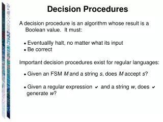
Reminder: DPLL-T • Our goal is to solve SMT problems with formulas from a theory T • DPLL-T is the most common approach • Based on the DPLL algorithm for SAT problems • Combines a decision procedure for the theory T
Linear Arithmetic • Theory grammar: • Can be defined over Rational () or Integers () • Example:
Why is it needed? Given the following C code: The following assembly can be generated:
Why is it needed? • A possible optimization: • Read the value of a[j] only once • Need to verify that loop won’t change a[j] • Can be encoded as Linear Arithmetic problem • If no solution is found, optimization is safe
Decision Procedures for • Gaussian’s elimination • Fourier-Motzkin • Simplex
Gaussian’s elimination • A simple method for solving a set of equalities • Less suitable for inequalities • Given a linear system Ax = b A x = b
Gaussian’s elimination • Manipulate A|b to an upper-triangular form • Then, solve backwards from the k’s row according to:
Gaussian elimination - example And now… x3 = -1, x2 = 3, x1 = 1 problem solved.
Fourier-Motzkin Elimination • Earliest method for solving linear inequalities • Given linear non-strict inequalities: • Pick a variable and eliminate it • Continue until all variables but one are eliminated • If problem included equalities, eliminate by assignment
A system of conjoined linear inequalities Fourier-Motzkin Elimination mconstraints nvariables
Fourier-Motzkin Elimination • When eliminating xn, partition the constraints according to the coefficient ain: • ain > 0: upper bound • ain < 0: lower bound assumeai,n >0
Fourier-Motzkin Elimination • Example: (1) x1 – x2 ≤ 0 (2) x1 – x3 ≤ 0 (3) -x1 + x2 + 2x3 ≤ 0 (4) -x3 ≤ -1 Category? Upper bound Assume we eliminatex1. Upper bound Lower bound
Fourier-Motzkin Elimination • For each pair of a lower bound aln<0 andupper bound aun>0, we have • For each such pair, add a constraint
Fourier-Motzkin Elimination • Example: (1) x1 – x2 ≤ 0 (2) x1 – x3 ≤ 0 (3) -x1 + x2 + 2x3 ≤ 0 (4) -x3 ≤ -1 (5) 2x3 ≤ 0 (from 1 and 3) (6) x2 + x3 ≤ 0 (from 2 and 3) We eliminatex1.
Fourier-Motzkin Elimination • Example: (1) x1 – x2 ≤ 0 (2) x1 – x3 ≤ 0 (3) -x1 + x2 + 2x3 ≤ 0 (4) -x3 ≤ -1 (5) 2x3 ≤ 0 (from 1 and 3) (6) x2 + x3 ≤ 0 (from 2 and 3) (7) 0 ≤ -1 (from 4 and 5) We eliminatex3. Contradiction (the system is unsatisfiable)!
Complexity of Fourier-Motzkin • Worst-case complexity: m2n • Popular in compilers • Because of simplicity • Popular when the problems are small – then it can be the fastest. • Not suitable for large problems • Need another solution for big problems
Simplex • Simplex was originally designed for solving optimization problems: • Given coefficient matrix and bound vector find a satisfying assignment that maximizes a goal function described by • Also known as Linear Programming • We are only interested in the feasibility problem • If problem is feasible than it is satisfiable
General form • Given same input as Fourier-Motzkin, convert input to general form • General form: • A combination of: • Linear equalities of the form • Lower and upper bounds on variables.
Converting to General Form • Replace (where )with and • s1,..., sm are called the additional variables.
Example 1 • Convertto:
Example 2 • Convertto:
Matrix form • Due to the additional variables: • now A is an mx (n + m) matrix. xy s1 s2 s3
xy s1 s2 s3 xy s1 s2 s3 The tableau • The diagonal part is inherent to the general form • Marked section will always be there • We can instead write:
xy s1 s2 s3 The tableau • The tableau changes throughout the algorithm, but maintains its m x n structure • Distinguish between basic and nonbasic variables • Initially, basic variables = the additional variables.
The tableau • Denote by • B– Basic variables • N – Nonbasic variables • The tableau is simply a rewrite of the system: • The basic variables are also called the dependent variables. • Their value is determined by the values of the other variables
The general simplex algorithm • Simplex maintains and updates: • The tableau, • an assignment to all variables • The bounds • Two invariants: • All nonbasic variables satisfy their bounds
Invariants • Initially, • B = additional variables • N = problem variables • (xi) = 0 for i {1,...,n+m} • Trivial to see that initial state satisfies invariants
The simplex algorithm • The initial assignment satisfies • If the bounds of all basic variables are satisfied by , return `Satisfiable’ • Otherwise... choose a variable and pivot • Pivoting is the basic step of the algorithm
Pivoting • Find a basic variable xithat violates its bounds. • Suppose that (xi) < li • We need to fix the value ofxi • Find a nonbasic variable xj such that • aij > 0 and(xj) < uj, or • aij < 0 and(xj) > lj • Such a variable xj is called suitable. • If there is no suitable variable – return ‘Unsatisfiable’
Pivoting xiwithxj • Solve equation i for xj: From: To: • Swap xi and xj, and update the i-th row accordingly. From To:
Pivoting xi withxj • Update all other rows: • Replace xjwith its equivalent obtained from row i:
Pivoting • Update as follows: • Increase (xj) by • Now xj is a basic variable: it can violate its bounds. • Update (xi) to li • Update for all other basic (dependent) variables.
Example • Recall the tableau and constraints in our example: • Initially assigns 0 to all variables • Bounds of s1 and s3 are violated
Example • Recall the tableau and constraints in our example: • We will pivot on s1 • x is a suitablenonbasic variable for pivoting • It has no upper bound • So now we pivot s1 with x
Example • Recall the tableau and constraints in our example: • Solve 1st row for x: • Replace x with s1 in other rows:
Example • The new state: • Solve 1st row for x: • Replace x with s1 in other rows:
Example • The new state: • We should increase x by • Hence, (x) = 0 + 2 = 2 • Now s1is equal to its lower bound: (s1) = 2 • Update all the others
Example • The new state: • Now s3 violates its lower bound • yis a suitable nonbasic variable for pivoting
Example • The new state: • We should increase y by
Example • The final state: • All constraints are now satisfied
A few observations • The additional variables: • Only additional variables have bounds. • These bounds are permanent. • Additional variables exit the base only on extreme points (their lower or upper bounds). • When entering the base, they shift towards the other bound and possibly cross it (violate it).
A few observations • Can it be that we pivot(xi,xj) and then pivot(xj,xi) and enter a (local) cycle ? • No. • Is termination guaranteed ? • No. • Perhaps there are bigger cycles.
A few observations • In order to avoid circles, we use Bland’s rule: • determine a total order on the variables. • Choose the first basic variable that violates its bounds, and first nonbasic suitable variable for pivoting. • It can be proven that this guarantees that no base is repeated, which implies termination. • We won’t prove this
A few observations • Simplex is exponential in the worst case • However, considered very efficient on most real practical problems • Need for exponential number of steps is rare
Decision Procedures for • Decision problem for is NP-hard • Unlike • Branch & Bound • Cuts • Omega test • Based on Fourier-Motzkin elimination • Will not be discussed today
Decision Procedures for • Both Branch & Bound and Cuts rely on a solver to provide a (possibly non-integer) solution • For example: Simplex • All variables in the final solution must be integers • In the case of simplex, this does not includes the additional variables • The additional variables do not have to be a part of the outputted solution