Comparing Groups – Part 2
Comparing Groups – Part 2. Wilcoxon Signed Rank (again). H 0 : θ = 0 H A : θ ≠ 0. θ represents the population mean or median. or in colors… add up the rank_AbsDiff for the green negative scores.

Comparing Groups – Part 2
E N D
Presentation Transcript
H0: θ = 0 HA: θ≠ 0 θ represents the population mean or median
or in colors… add up the rank_AbsDiff for the green negative scores or in colors… add up the rank_AbsDiff for the blue positive scores
or in colors… add up the rank_AbsDiff for the green negative scores R- = 1.5 + 3 + 4.5 + 4.5+ 7.5 + 7.5+7.5+14.5+18.5 = 64.5 or in colors… add up the rank_AbsDiff for the blue positive scores R+ = 1.5 + 7.5 + 11 +11 +11 +14.5 +14.5 +14.5+18.5+18.5+18.5+21+22= 188.5 188.5-64.5/2=62
One-way ANOVA in R • In the last lecture I gave you a demonstration of using SAS to conduct a one-way ANOVA. Many people think that R is a superior tool for doing analyses like ANOVA. While R is not critical for simple models like you have seen, it is invaluable for graphics to describe more complicated models.
R and Anxiety Disorders • Start R and then type library(Rcmdr) • Load the dataset using the Import Data option on the Data menu. • Load the Generalized Anxiety Disorder (GAD) data. It has Hamilton Rating Scale for Anxiety data for people taking placebo, high or low dose drug.
Show me the means. • You want to see if there is a difference in means in the 3rd variable for the levels of the 2nd variable. You can request the mean plot:
The Plot of the Design I really like boxplots to see the variability around these means.
Gad <- na.omit(Gad) plot.design(Gad[, c(2,3)]) attach(Gad) thePlot = (boxplot(HAMA~DOSEGRP, ylab="HAMA", xlab="DOSEGRP")) where = seq(thePlot$n) theMeans = tapply(HAMA, DOSEGRP, mean) points(where, theMeans, col = "red", pch = 18) I want means.
Testing for Differences • Once the data is set with the placebo group as the baseline, it is easy to ask for tests for the differences vs. the baseline level.
General Linear Models • It is important for you to know that ANOVAs are more than stand-alone analyses that are not related to modeling. ANOVA fits into a class of statistics called General Linear Models. They are well implemented in R and Rcmdr.
Checking the Model • With the working model you can get lots of summary information, including diagnostic plots.
More Advanced Contrasts • There is a plethora of methods for dealing with multiple comparisons. You can search CRAN for specific methods you see in textbooks. For example, Walker uses Dunnett’s T test for contrasting the placebo vs. the other levels. • I start search CRAN with RSiteSearch(“blah”)
Nasty code…. • I eventually found the method implemented in a package called multcomp: library(multcomp) gad.aov = aov(HAMA ~ DOSEGRP, data = Gad) summary(glht(gad.aov, linfct = mcp(DOSEGRP="Dunnett"))) confint(glht(gad.aov, linfct = mcp(DOSEGRP="Dunnett")))
Two-Way ANOVA • When you have two or more predictors, you want to know if the variables impact the outcome means by themselves and also if they interact. If variables interact, it means that together they do things to the outcome variable beyond what you would expect from looking at each variable alone. For example, smoking and eating too much both hurt longevity but the combination of the two factors may not be as bad as expected or the combination may be especially lethal.
Anemia • People with Cervical (C), Prostate(P) or Colorectal (R) cancers with chemotherapy-induced anemia were treated either with a drug or placebo and the changes in their hemoglobin levels were assessed. The question of interest is, does the drug reduce anemia?
Box Plots of Course • With code or R commander get boxplots for the levels of the predictors:
Design Plots • You have analysis variables in columns 1, 2 and 4. So specify the design plot like this:
Interaction Plots • In addition to the main effects for the predictors, you want to see if the drug behaves differently in the people with the three different cancer groups. Perhaps it helps increase hemoglobin in one group and decreases it another. Type your outcome variable last.
It looks like there are differences between the cancer types and the drug seems to increase the hemoglobin relative to the placebo.
Modeling Anova with a capital A is part of the car package
Results To turn off the * stuff, type this code before you model: options(show.signif.stars=FALSE)
ANOVA as a Model • You can build this ANOVA as a linear model.
used for nesting y ~ A/B y ~ A + A:B y ~ A + B % in % A interaction only main effect and interaction Set interaction limits (A+B+C) ^ 2 is equal to A*B*C - A:B:C Main effect Remove an explanatory effect.
SAS EG example • See the parallel information in the SAS EG project.