Download
1 / 39
390 likes | 540 Vues
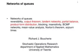
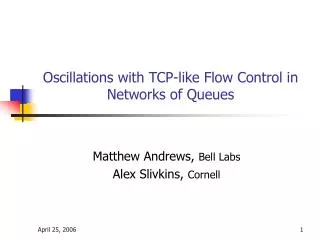
Oscillations with TCP-like Flow Control in Networks of Queues. Matthew Andrews, Bell Labs Alex Slivkins, Cornell. Network Utility Maximization. Wireline networks max i U i (x i ) subject to . Q i x i c Q x i = inj rate into path i

E N D
Oscillations with TCP-like Flow Control in Networks of Queues Matthew Andrews, Bell Labs Alex Slivkins, Cornell
Network Utility Maximization • Wireline networks max i Ui(xi) subject to . Q i xi cQ • xi = inj rate into path i • cQ = capacity of server Q • Ui(.) = utility function (e.g. log) • Kelly-Maulloo-Tan, Low-Lapsley, Low-Peterson-Wang… • “TCP is a primal dual algorithm for solving this problem” S2 S3 S1 t1 server A server B t2 t3
Example • Kelly, Maulloo, Tan • xi (t) = injection rate into flow i at time t • pQ = price for congestion at router Q
Network Utility Maximization • Wireless networks max i Ui(xi) subject to . ( …, xi , … ) C • C = system capacity region (convex) • Depends on power assignments, interference etc. • Chiang • Joint power control and congestion control for solving problem
Convergence vs oscillations Inj rate x2 Inj rate x3 S2 S3 Inj rate x1 Server B S1 t1 Server A Cong at server A = x1 + x2 t2 t3 • Prior work: • Congestion of server Q = F(injection rates of flows that use Q) • For example, congestion is signaled before queues buildup (e.g. via ECN) • Arrival rate of flow at server = flow injection rate • Allows for convergence results
Convergence vs oscillations S2 S1 S3 t2 t3 • This talk • Suppose congestion causes queue buildups • Flow arrival rate at server not necessarily equal to flow injection rate • Do convergence results still hold? t1
t1 t2 t3 Sending rates vs arrival rates inji(t) • due to queues that are upstream,in general arrival rates arr1(t), arr2(t), arr3(t)are different from sending rates inj1(t), inj2(t), inj3(t) • Suppose we use the true arrival rates • i.e. cong =arr1(t) + arr2(t) + arr3(t) S1 S2 S3 arri(t) server
Convergence vs oscillations • Result: for any TCP-like congestion control mechanism,there exists a network of (wireline) servers and a set of flows such that starting from a certain initial state, system oscillates in a suboptimal state at all times, for each server, the total sending rate of all flows that use this server is less than its capacity
S2 S3 S1 t1 router router t2 t3 Convergence vs oscillations • Prior work: for a version of TCP, system converges to a social optimumstarting from any initial state • [Kelly, Maulloo, Tan ’98] + follow-ups • approximation of FIFO dynamics • Our contribution: for any TCP-like congestion control mechanism,there exists a network of routers and a set of sessions such thatstarting from a certain initial state, system oscillates at all times, for each router, the total sending rate of all sessions that use this router is less than its capacity
?? • no congestion: all queues are empty S S t t • congestion: at least one queue is non-empty Parameterized congestion control • sender detects congestion using feedback from receiver • yes decrease sending rate; noincrease sending rate
Parameterized congestion control • sender detects congestion using feedback from receiver • yes decrease sending rate; noincrease sending rate • discrete-time TCP: additive increase, multiplicative decrease • yes decrease rate by half; noincrease rate by 1 • we use a continuous-time approximation • yes congestion sending rate f(t) = f(0) et • nocongestion sending rate g(t) = g(0)+ t • is the damping parameter that controls the rate of change • generalization: (almost) any flow increase function g(t), any f(t) that satisfies some axioms, e.g. f(t) = f(0) t
we are extending our construction to the all-FIFO case Main result Theorem For any given congestion control {f(t), g(t)} there exists: • damping parameter (same for all sessions) • a network of routers, a set of sessions, and an initial state such that system oscillates and for each router, the total sending rate of all sessions that use this router is always less than its capacity Note routers are almost FIFO: • each session is in one of the two priority classes • FIFO scheduling for sessions within the same class
start Q1 Q1 Q1 Q2 Q2 Q2 Q3 Q3 Q3 Q4 Q4 Q4 S S S t t t 1 finish 1 The basic gadget: high-level idea capacity 1 <1 <1 1
init rate S’ capacity 1 <1 <1 1 init rate 0 1 t’ The basic gadget: animation Q1 Q2 Q3 Q4 S t
capacity 1 <1 <1 1 Q1 Q2 Q3 Q4 S t The basic gadget: animation init rate S’ rate = 0 t’
capacity 1 <1 <1 1 Q1 Q2 Q3 Q4 S t rate The basic gadget: animation S’ rate = 0 t’
capacity 1 <1 <1 1 Q1 Q2 Q3 Q4 S t The basic gadget: animation rate = 0 S’ rate = 0 1 t’
rate capacity 1 <1 <1 1 Q1 Q2 Q3 Q4 S t The basic gadget: animation S’ rate = 0 t’
before 1 1 2 2 3 3 4 4 • after 1 2 3 1 2 3 4 Connect two gadgets identify Q4 from one gadget with Q1 from another
1 2 3 1 2 3 1 2 3 1 2 3 Row of gadgets rate 0 rate e rate e rate e S1 t1
1 2 3 1 2 3 1 2 3 1 2 3 Row of gadgets rate e rate 0 rate e rate e S1 t1
1 2 3 1 2 3 1 2 3 1 2 3 Row of gadgets rate e rate e rate 0 rate e S1 t1
1 2 3 1 2 3 1 2 3 1 2 3 Row of gadgets rate e rate e rate e rate 0 S1 t1 fluid eventually reaches its destination, and the process stopsnot too exciting!
rate 0 rate 0 rate 0 rate e rate e rate e rate 0 1 2 3 1 2 3 1 2 3 1 2 3 Row of gadgets S1 t1 a better process
rate 0 rate 0 rate 0 rate e rate e rate e rate 0 1 2 3 1 2 3 1 2 3 1 2 3 refill Row of gadgets and now a refill happens S1 t1 a better process
refill 1 2 3 1 2 3 1 2 3 1 2 3 Row of gadgets ... and so on S1 t1 a better process
S1 t1 1 1 1 2 2 2 3 3 3 1 1 1 2 2 2 3 3 3 1 1 1 2 2 2 3 3 3 1 1 1 2 2 2 3 3 3 S2 t2 S3 t3 Rows of gadgets each row is running the same process, shifted in time
refill S1 t1 1 1 1 2 2 2 3 3 3 1 1 1 2 2 2 3 3 3 1 1 1 2 2 2 3 3 3 1 1 1 2 2 2 3 3 3 refill S2 t2 refill S3 t3 Rows of gadgets now a refill happens each row is running the same process, shifted in time
refill S1 t1 1 1 1 2 2 2 3 3 3 1 1 1 2 2 2 3 3 3 1 1 1 2 2 2 3 3 3 1 1 1 2 2 2 3 3 3 S2 t2 S3 t3 Rows of gadgets ... and so on Wait a sec... how do the refills happen ???
S1 t1 1 1 1 1 2 2 2 2 3 3 3 3 1 1 1 1 2 2 2 2 3 3 3 3 1 1 1 1 2 2 2 2 3 3 3 3 1 1 1 1 2 2 2 2 3 3 3 3 S2 t2 S3 t3 S4 t4 Refills and vertical sessions rate >0
S1 t1 1 1 1 1 2 2 2 2 3 3 3 3 1 1 1 1 2 2 2 2 3 3 3 3 1 1 1 1 2 2 2 2 3 3 3 3 1 1 1 1 2 2 2 2 3 3 3 3 S2 t2 S3 t3 S4 t4 Refills and vertical sessions rate >0
S1 t1 1 1 1 1 2 2 2 2 3 3 3 3 1 1 1 1 2 2 2 2 3 3 3 3 1 1 1 1 2 2 2 2 3 3 3 3 1 1 1 1 2 2 2 2 3 3 3 3 S2 t2 S3 t3 S4 t4 Refills and vertical sessions rate >0
S1 t1 1 1 1 1 2 2 2 2 3 3 3 3 1 1 1 1 2 2 2 2 3 3 3 3 1 1 1 1 2 2 2 2 3 3 3 3 1 1 1 1 2 2 2 2 3 3 3 3 S2 t2 S3 t3 rate S4 t4 Refills and vertical sessions
S1 t1 1 1 1 1 2 2 2 2 3 3 3 3 1 1 1 1 2 2 2 2 3 3 3 3 1 1 1 1 2 2 2 2 3 3 3 3 1 1 1 1 2 2 2 2 3 3 3 3 S2 t2 S3 t3 S4 t4 Refills and vertical sessions refilled !!! rate = 0
Joint scheduling + cong control xi xj • Solution: do joint scheduling and congestion control. • Problem definition • Model queues explicitly • When data served by one server, passes to next server on flow route • Design scheduling + cong control max i Ui(xi) subject to . All queues are stable
Joint scheduling + cong control xi xj • Greedy Primal Dual Algorithm (Stolyar) • Simple version • Flow Routes are given • Set of routes to destination d form rooted tree • At most 1 pckt into each flow per time step • Per destination queues • Qv,d = amount of dest d data at node v • nv,d = next hop for Qv,d data • rv,w(t) = data rate between nodes v,w
Joint scheduling + cong control xi xj • Greedy Primal Dual Algorithm • Scheduling • Node v serves data from queue that maximizes (Qv,d – Qnv,d,d) rv,nv,d(t) • Congestion control • Flow i injects a packet whenever U’(xi(t)) – b.Qibegin > 0 b = small parameter Qibegin = first queue on path of flow i
Joint scheduling + cong control xi xj • Greedy Primal Dual Algorithm • Solves the utility maximization problem max i Ui(xi) subject to . All queues are stable • Works for wireless networks • Joint scheduling and cong control • Collaboration via queues sizes • Do not get excessive queue buildup • Scheduling creates “backpressure”
Conclusions and open questions End-to-end congestion control can cause oscillations when interacting with network of queues running simple scheduling policies • solution: tighter integration of scheduling and congestion control,e.g. Greedy Primal-Dual algorithm of Sasha Stolyar Related work due to Eryilmaz-Srikant and Neely-Modiano-Li Our example is paranoid, but we need to replicate initial state exactly • our result suggests that in practice convergence can be hard, too Open questions: • extension to the all-FIFO case • non-FIFO schedulers, e.g. Generalized Processor Sharing