Solver Settings
Solver Settings. Outline. Using the Solver Setting Solver Parameters Convergence Definition Monitoring Stability Accelerating Convergence Accuracy Grid Independence Adaption Appendix: Background Finite Volume Method Explicit vs. Implicit Segregated vs. Coupled Transient Solutions.

Solver Settings
E N D
Presentation Transcript
Outline • Using the Solver • Setting Solver Parameters • Convergence • Definition • Monitoring • Stability • Accelerating Convergence • Accuracy • Grid Independence • Adaption • Appendix: Background • Finite Volume Method • Explicit vs. Implicit • Segregated vs. Coupled • Transient Solutions
Set the solution parameters Initialize the solution Enable the solution monitors of interest Calculate a solution Modify solution parameters or grid Check for convergence No Yes Yes Check for accuracy Stop No Solution Procedure Overview • Solution Parameters • Choosing the Solver • Discretization Schemes • Initialization • Convergence • Monitoring Convergence • Stability • Setting Under-relaxation • Setting Courant number • Accelerating Convergence • Accuracy • Grid Independence • Adaption
Choosing a Solver • Choices are Coupled-Implicit, Coupled-Explicit, or Segregated (Implicit) • The Coupled solvers are recommended if a strong inter-dependence exists between density, energy, momentum, and/or species. • e.g., high speed compressible flow or finite-rate reaction modeled flows. • In general, the Coupled-Implicit solver is recommended over the coupled-explicit solver. • Time required: Implicit solver runs roughly twice as fast. • Memory required: Implicit solver requires roughly twice as much memory as coupled-explicit or segregated-implicit solvers! • The Coupled-Explicit solver should only be used for unsteady flows when the characteristic time scale of problem is on same order as that of the acoustics. • e.g., tracking transient shock wave • The Segregated (implicit) solver is preferred in all other cases. • Lower memory requirements than coupled-implicit solver. • Segregated approach provides flexibility in solution procedure.
Discretization (Interpolation Methods) • Field variables (stored at cell centers) must be interpolated to the faces of the control volumes in the FVM: • FLUENT offers a number of interpolation schemes: • First-Order Upwind Scheme • easiest to converge, only first order accurate. • Power Law Scheme • more accurate than first-order for flows when Recell< 5 (typ. low Re flows). • Second-Order Upwind Scheme • uses larger ‘stencil’ for 2nd order accuracy, essential with tri/tet mesh or when flow is not aligned with grid; slower convergence • Quadratic Upwind Interpolation (QUICK) • applies to quad/hex and hyrbid meshes (not applied to tri’s), useful for rotating/swirling flows, 3rd order accurate on uniform mesh.
Interpolation Methods for Pressure • Additional interpolation options are available for calculating face pressure when using the segregated solver. • FLUENTinterpolation schemes for Face Pressure: • Standard • default scheme; reduced accuracy for flows exhibiting large surface-normal pressure gradients near boundaries. • Linear • use when other options result in convergence difficulties or unphysical behavior. • Second-Order • use for compressible flows; not to be used with porous media, jump, fans, etc. or VOF/Mixture multiphase models. • Body Force Weighted • use when body forces are large, e.g., high Ra natural convection or highly swirling flows. • PRESTO! • use on highly swirling flows, flows involving porous media, or strongly curved domains.
Pressure-Velocity Coupling • Pressure-Velocity Coupling refers to the way mass continuity is accounted for when using the segregated solver. • Three methods available: • SIMPLE • default scheme, robust • SIMPLEC • Allows faster convergence for simple problems (e.g., laminar flows with no physical models employed). • PISO • useful for unsteady flow problems or for meshes containing cells with higher than average skew.
Initialization • Iterative procedure requires that all solution variables be initialized before calculating a solution. Solve Initialize Initialize... • Realistic ‘guesses’ improves solution stability and accelerates convergence. • In some cases, correct initial guess is required: • Example: high temperature region to initiate chemical reaction. • “Patch” values for individualvariables in certain regions. Solve Initialize Patch... • Free jet flows(patch high velocity for jet) • Combustion problems(patch high temperaturefor ignition)
Convergence Preliminaries: Residuals • Transport equation for f can be presented in simple form: • Coefficients ap, anbtypically depend upon the solution. • Coefficients updated each iteration. • At the start of each iteration, the above equality will not hold. • The imbalance is called the residual, Rp, where: • Rp should become negligible as iterations increase. • The residuals that you monitor are summed over all cells: • By default, the monitored residuals are scaled. • You can also normalize the residuals. • Residuals monitored for the coupled solver are based on the rms value of the time rate of change of the conserved variable. • Only for coupled equations; additional scalar equations use segregated definition.
Convergence • At convergence: • All discrete conservation equations (momentum, energy, etc.) are obeyed in all cells to a specified tolerance. • Solution no longer changes with more iterations. • Overall mass, momentum, energy, and scalar balances are obtained. • Monitoring convergence with residuals: • Generally, a decrease in residuals by 3 orders of magnitude indicates at least qualitative convergence. • Major flow features established. • Scaled energy residual must decrease to 10-6 for segregated solver. • Scaled species residual may need to decrease to 10-5 to achieve species balance. • Monitoring quantitative convergence: • Monitor other variables for changes. • Ensure that property conservation is satisfied.
All equations converged. 10-3 10-6 Convergence Monitors: Residuals • Residual plots show when the residual values have reached the specified tolerance. Solve Monitors Residual...
Convergence Monitors: Forces/Surfaces • In addition to residuals, you can also monitor: • Lift, drag, or moment Solve Monitors Force... • Variables or functions (e.g., surface integrals)at a boundary or any defined surface: Solve Monitors Surface...
Checking for Property Conservation • In addition to monitoring residual and variable histories, you should also check for overall heat and mass balances. • At a minimum, the net imbalance should be less than 1% of smallest flux through domain boundary. ReportFluxes...
Decreasing the Convergence Tolerance • If your monitors indicate that the solution is converged, but the solution is still changing or has a large mass/heat imbalance: • Reduce Convergence Criterionor disable Check Convergence. • Then calculate until solutionconverges to the new tolerance.
Continuity equation convergence trouble affects convergence of all equations. Convergence Difficulties • Numerical instabilities can arise with an ill-posed problem, poor quality mesh, and/or inappropriate solver settings. • Exhibited as increasing (diverging) or “stuck” residuals. • Diverging residuals imply increasing imbalance in conservation equations. • Unconverged results can be misleading! • Troubleshooting: • Ensure problem is well posed. • Compute an initial solution witha first-order discretization scheme. • Decrease under-relaxation for equations having convergence trouble (segregated). • Reduce Courant number (coupled). • Re-mesh or refine grid with high aspect ratio or highly skewed cells.
Modifying Under-relaxation Factors • Under-relaxation factor, , is included to stabilize the iterative process for the segregated solver. • Use default under-relaxation factors to start a calculation. Solve Controls Solution... • Decreasing under-relaxation for momentum often aids convergence. • Default settings are aggressive but suitable for wide range of problems. • ‘Appropriate’ settings best learned from experience. • For coupled solvers, under-relaxation factors for equations outside coupled set are modified as in segregated solver.
Modifying the Courant Number • Courant number defines a ‘time step’ size for steady-state problems. • A transient term is included in the coupled solver even for steady state problems. • For coupled-explicit solver: • Stability constraints impose a maximum limit on Courant number. • Cannot be greater than 2. • Default value is 1. • Reduce Courant number when having difficulty converging. • For coupled-implicit solver: • Courant number is not limited by stability constraints. • Default is set to 5.
Accelerating Convergence • Convergence can be accelerated by: • Supplying good initial conditions • Starting from a previous solution. • Increasing under-relaxation factors or Courant number • Excessively high values can lead to instabilities. • Recommend saving case and data files before continuing iterations. • Controlling multigrid solver settings. • Default settings define robust Multigrid solver and typically do not need to be changed.
Starting from a Previous Solution • Previous solution can be used as an initial condition when changes are made to problem definition. • Once initialized, additional iterations uses current data set as starting point.
fine (original) mesh ‘solution transfer’ coarse mesh Multigrid • The Multigrid solver accelerates convergence by using solution on coarse mesh as starting point for solution on finer mesh. • Influence of boundaries and far-away points are more easily transmitted to interior of coarse mesh than on fine mesh. • Coarse mesh defined from original mesh. • Multiple coarse mesh ‘levels’ can be created. • AMG- ‘coarse mesh’ emulated algebraically. • FAS- ‘cell coalescing’ defines new grid. • a coupled-explicit solver option • Final solution is for original mesh. • Multigrid operates automatically in the background. • Accelerates convergence for problems with: • Large number of cells • Large cell aspect ratios, e.g., x/y > 20 • Large differences in thermal conductivity
Accuracy • A converged solution is not necessarily an accurate one. • Solve using 2nd order discretization. • Ensure that solution is grid-independent. • Use adaption to modify grid. • If flow features do not seem reasonable: • Reconsider physical models and boundary conditions. • Examine grid and re-mesh.
Mesh Quality and Solution Accuracy • Numerical errors are associated with calculation of cell gradients and cell face interpolations. • These errors can be contained: • Use higher order discretization schemes. • Attempt to align grid with flow. • Refine the mesh. • Sufficient mesh density is necessary to resolve salient features of flow. • Interpolation errors decrease with decreasing cell size. • Minimize variations in cell size. • Truncation error is minimized in a uniform mesh. • Fluent provides capability to adapt mesh based on cell size variation. • Minimize cell skewness and aspect ratio. • In general, avoid aspect ratios higher than 5:1 (higher ratios allowed in b.l.). • Optimal quad/hex cells have bounded angles of 90 degrees • Optimal tri/tet cells are equilateral.
Determining Grid Independence • When solution no longer changes with further grid refinement, you have a “grid-independent” solution. • Procedure: • Obtain new grid: • Adapt • Save original mesh before adapting. • If you know where large gradients are expected, concentrate the original grid in that region, e.g., boundary layer. • Adapt grid. • Data from original grid is automatically interpolated to finer grid. • file write-bc and file read-bc facilitates set up of new problem • file reread-grid and File Interpolate... • Continue calculation to convergence. • Compare results obtained w/different grids. • Repeat procedure if necessary.
Unsteady Flow Problems • Transient solutions are possible with both segregated and coupled solvers. • Solver iterates to convergence at each time level, then advances automatically. • Solution Initialization defines initial condition and must be realistic. • For segregated solver: • Time step size, t, is input in Iterate panel. • t must be small enough to resolve time dependent features and to ensure convergence within 20 iterations. • May need to start solution with small t. • Number of time steps, N, is also required. • N*t = total simulated time. • To iterate without advancing time step, use ‘0’ time steps. • PISO may aid in accelerating convergence for each time step.
Unsteady Modeling Options • Adaptive Time Stepping • Controls how time step size changes. • User-Defined inputs also available. • Time averaged data may be acquired. • Particularly useful for LES turbulence modeling. • If desirable, animations should be set up before iterating (flow visualization). • For Coupled Solver, Courant number defines in practice: • global time step size for coupled explicit solver. • pseudo-time step size for coupled implicit solver. • Real time step size must still be defined.
Summary • Solution procedure for the segregated and coupled solvers is the same: • Calculate until you get a converged solution. • Obtain second-order solution (recommended). • Refine grid and recalculate until grid-independent solution is obtained. • All solvers provide tools for judging and improving convergence and ensuring stability. • All solvers provide tools for checking and improving accuracy. • Solution accuracy will depend on the appropriateness of the physical models that you choose and the boundary conditions that you specify.
Appendix • Background • Finite Volume Method • Explicit vs. Implicit • Segregated vs. Coupled • Transient Solutions
unsteady convection generation diffusion control volume Fluid region of pipe flow discretized into finite set of control volumes (mesh). Background: Finite Volume Method - 1 • FLUENT solvers are based on the finite volume method. • Domain is discretized into a finite set of control volumes or cells. • General transport equation for mass, momentum, energy, etc. is applied to each cell and discretized. For cell p, • All equations are solved to render flow field.
face f cell p adjacent cells, nb Background: Finite Volume Method - 2 • Each transport equation is discretized into algebraic form. For cell p, • Discretized equations require information at cell centers and faces. • Field data (material properties, velocities, etc.) are stored at cell centers. • Face values can be expressed in terms of local and adjacent cell values. • Discretization accuracy depends upon ‘stencil’ size. • The discretized equation can be expressed simply as: • Equation is written out for every control volume in domain resulting in an equation set.
Background: Linearization • Equation sets are solved iteratively. • Coefficients ap and anb are typically functions of solution variables(nonlinear and coupled). • Coefficients are written to use values of solution variables from previous iteration. • Linearization: removing coefficients’ dependencies on . • De-coupling: removing coefficients’ dependencies on other solution variables. • Coefficients are updated with each iteration. • For a given iteration, coefficients are constant. • p can either be solved explicitly or implicitly.
Background: Explicit vs. Implicit • Assumptions are made about the knowledge of nb: • Explicit linearization - unknown value in each cell computed from relations that include only existing values (nb assumed known from previous iteration). • p solved explicitly usingRunge-Kutta scheme. • Implicit linearization - pandnb are assumed unknown and are solved using linear equation techniques. • Equations that are implicitly linearized tend to have less restrictive stability requirements. • The equation set is solved simultaneously using a second iterative loop (e.g., point Gauss-Seidel).
Background: Coupled vs. Segregated • Segregated Solver • If the only unknowns in a given equation are assumed to be for a single variable, then the equation set can be solved without regard for the solution of other variables. • coefficients ap and anb are scalars. • Coupled Solver • If more than one variable is unknown in each equation, and each variable is defined by its own transport equation, then the equation set is coupled together. • coefficients ap and anb are Neqx Neq matrices • is a vector of the dependent variables, {p, u, v, w, T, Y}T
Update properties. Solve momentum equations (u, v, w velocity). Solve pressure-correction (continuity) equation.Update pressure, face mass flow rate. Solve energy, species, turbulence, and other scalar equations. Converged? No Yes Stop Background: Segregated Solver • In the segregated solver, each equation is solved separately. • The continuity equation takes the form of a pressure correction equation as part of SIMPLE algorithm. • Under-relaxation factors are included in the discretized equations. • Included to improve stability of iterative process. • Under-relaxation factor, , in effect, limits change in variable from one iteration to next:
Update properties. Solve continuity, momentum, energy, and species equations simultaneously. Solve turbulence and other scalar equations. Converged? Yes No Stop Background: Coupled Solver • Continuity, momentum, energy, and species are solved simultaneously in the coupled solver. • Equations are modified to resolve compressible and incompressible flow. • Transient term is always included. • Steady-state solution is formed as time increases and transients tend to zero. • For steady-state problem, ‘time step’ is defined by Courant number. • Stability issues limit maximum time step size for explicit solver but not for implicit solver. CFL= Courant-Friedrichs-Lewy-number where u = appropriate velocity scale x = grid spacing
Coupled Solver Discretization of: pseudo-time Implicit Explicit Steady Unsteady Steady Unsteady Dt Dt physical-time Implicit Implicit Explicit Dt Dt, Dt Dt, Dt (global time step) Background: Coupled/Transient Terms • Coupled solver equations always contain a transient term. • Equations solved using the unsteady coupled solver may contain two transient terms: • Pseudo-time term, Dt. • Physical-time term, Dt. • Pseudo-time term is driven to near zero at each time step and for steady flows. • Flow chart indicates which time step size inputs are required. • Courant number defines Dt • Inputs to Iterate panel define Dt.