Download
1 / 16
160 likes | 285 Vues
This document outlines the essential cartographic requirements for converting image objects into maps within the GEOBIA framework. It emphasizes the importance of imagery data quality, spatial resolution, and the removal of representational artifacts to meet cartographic accuracy. The paper discusses constraints imposed by image resolution and human visual acuity, proposing methods for simplifying data to adhere to map scale specifications. Additionally, it highlights the significance of addressing jagged outlines and maintaining visual clarity in the final cartographic output.

E N D
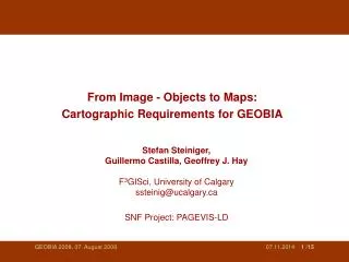
From Image - Objects to Maps: • Cartographic Requirements for GEOBIA Stefan Steiniger, Guillermo Castilla, Geoffrey J. Hay F3GISci, University of Calgary ssteinig@ucalgary.ca SNF Project: PAGEVIS-LD GEOBIA 2008, 07. August 2008
Outline • Objective • Requirements on Imagery Data • Removing Representational Artifacts • Introducing Scale: Cartographic Constraints • Conclusions & Outlook GEOBIA 2008, 07. August 2008
1. Objective • from image-objects to maps Map (map data 1:5k, City of Zurich) objects image (0.50m) • Objective:simplify GEOBIA results to ensure cartographic standards • Discuss: cartographic requirements imposed on data and their visualization GEOBIA 2008, 07. August 2008
. imagery needs a certain spatial resolution to fit the maps accuracy requirements! or conversely: . the image resolution defines the finest derivable map scale 2. Requirements on Image Data • . a map, as raster/vector graphics, has a defined • map scale (e.g. 1:25 000) • . the map scale imposes • 1. a minimal object size that can be displayed in [m], • 2. a positional accuracy How to establish the relationship between image resolution and map scale? » GEOBIA 2008, 07. August 2008
.Image: Nyquist-Shannon Sampling theorem: • need of at least 2 samples to re-construct a signal • (signal = an object in the image) • . we need (min): 4px for a house & 2 px for a road 2. Requirements on Image Data • .Map: human eye acuity: • ~ 0.2mm for reading distance of 30cm (SSC 2005, p.26) • .smallest map object that can be displayed: 0.2mm bringing things together » GEOBIA 2008, 07. August 2008
2. Requirements on Image Data • Example 1: • . required map scale: 1:25 000 • 0.2mm (acuity) = 2px (NS) • 0.2mm*25000 = 5m • 5m = 2px • . needed resolution at least 2.5m/px Nyquist Example 2: . image resolution: 0.5m/px . 2px = 1m = 0.2mm (map) . scale = 1.0m / 0.2mm = 1:5000+ Acuity: 0.2mm GEOBIA 2008, 07. August 2008
3. Removing Representational Artifacts • . three images taken from journal publications • .jaggedoutlines : an artifact from change of representation (R to V) • . side-effects: • . introducing a pseudo accuracy (psychological; metadata?) • . doesn’t look nice • let’s remove jagged lines! (e.g. simplification and/or smoothing) GEOBIA 2008, 07. August 2008
3. Removing Representational Artifacts • Example: 0.5 m/px Segmentation with Definiens (scale factor: 50) Smoothing (Snakes, 0.4m) Simplification (DP, 0.1m) GEOBIA 2008, 07. August 2008
Smoothing (Snakes, 0.4m) Simplification (DP, 0.1m) 3. Removing Representational Artifacts • note: maximal displacement of line is adjustable: 0.4m+0.1m = 0.5m = 1px • Example: 0.5 m/px Segmentation with Definiens (scale factor: 50) Smoothing (Snakes, 0.4m) Simplification (DP, 0.1m) GEOBIA 2008, 07. August 2008
Smoothing (Snakes, 0.8m) Simplification (DP, 0.2m) Smoothing (Snakes, 0.4m) Simplification (DP, 0.1m) 3. Removing Representational Artifacts • Example: 0.5 m/px Segmentation with Definiens (scale factor: 50) Smoothing (Snakes, 0.4m) Simplification (DP, 0.1m) GEOBIA 2008, 07. August 2008
4. Introducing Scale: Cartographic Constraints • Background: • . automated map generalization: “constraint-based” modeling (Beard 1991) • .constraint: condition to which the map should adhere (Weibel and Dutton 1998) • . several types of constraints: • . geometrical • . topological • . contextual • . cultural • . procedural • . with different objectives: • . ensure legibility (active) • . preserve shape + location Fig.: constraints on buildings GEOBIA 2008, 07. August 2008
4. Introducing Scale: Cartographic Constraints • . Galanda (2003): constraints on polygonal subdivisions • 1. geometrical constraints (active): • . minimal area • . object separation (e.g. holes) • . consecutive vertex distance* • . inner-width • . outline granularity • 2. procedural constraints • . redundant points (*) • 3. and other (preserving) constraints • . e.g. structure preservation [area & • class ratios] • . e.g. modeling related • . e.g. topological [self-intersection] Fig.: geometric constraints on polygons GEOBIA 2008, 07. August 2008
4. Introducing Scale: Cartographic Constraints • Example: • . image 0.5m/px • . segmented with SCRM • (Castilla et al. 2008) • . simplified (DP) & merged • . target map scale: 1:5.000 • .Result: polygon-parts • that do not fulfill the • constraints (min-dimension • SSC 2005: 0.4mm = 2m) result of constraint evaluation polygons from segmentation GEOBIA 2008, 07. August 2008
5. Conclusions and Outlook • Conclusions • To create maps from image objects we need to simplify these to ensure cartographic standards! • This requires to be aware of: • 1. the image resolution that constraints spatial accuracy • 2. jagged lines that should be removed • 3. cartographic constraints that account for human vision • Benefits: • 1. further the cartographic utility of GEOBIA results • 2. implicit data reduction facilitates further GIS analysis GEOBIA 2008, 07. August 2008
5. Conclusions and Outlook • Outlook • build an automated system that • 1. implements relevant cartographic constraints • 2. offers map generalization algorithms to fulfill these constraints • 3. detects patterns (based on spectral and geometric • information) to enable a meaningful aggregation of polygon • patches (segments) GEOBIA 2008, 07. August 2008
Thank you for your attention! • Acknowledgments: • Swiss National Science Foundation: Project PAGEVIS-LD • References: • . Beard (1991): Constraints on rule formation. In Map Generalization: Making Rules for Knowledge Representation, B. Buttenfield and R. McMaster (Eds), pp. 121–135 (London: Longman). • . Galanda (2003): Agent based generalization of polygonal data. Ph.D. thesis, Department of Geography, University of Zurich. • . SSC - Swiss Society of Cartography (2005): Topographic Maps – Map Graphics and Generalisation. Cartographic Publication Series, 17 (Berne: Federal Office of Topography) • . Weibel and Dutton (1998): Constraint-based automated map generalization. In Proceedings 8th International Symposium on Spatial Data Handling, Vancouver, Canada, pp. 214–224. GEOBIA 2008, 07. August 2008