Simulation Methods for Ensuring Target Service Levels in Inventory Systems
100 likes | 195 Vues
Research focuses on optimizing inventory systems with service level constraints using sample average approximation and sampling techniques.

Simulation Methods for Ensuring Target Service Levels in Inventory Systems
E N D
Presentation Transcript
Simulation Methods for Ensuring Target Service Levels in Inventory Systems CELDI Member: Invistics, Inc. Manuel D. Rossetti (PI), Yasin Ünlü (RA) Department of Industrial Engineering The University of Arkansas October 2010
Motivating Problem • Inventory policies are set to optimize operational performance measures subject to service constraints. • To calculate the operational performance, the modeling of the lead-time demand (LTD) is critical; however, the actual LTD model is difficult to directly measure in practice. • The modeling of the LTD model is often performed by assuming a distributional family (e.g . Normal, Poisson, etc.) • Estimates of parameters (e.g. mean and variance) based on forecast estimates and forecast error (or other knowledge) are used to represent the first two moments of the assumed distribution. • Once parameterized, the distribution is used in inventory optimization procedures. • The selection and representation of the LTD model based on two moment parameters can be very poor. • This causes inventory planning models to not adequately represent the actual performance. This results in riskier and possibly more costly inventory plans. • Thus, the problem is to develop an approach without relying on a LTD model • for policy optimization subject to a service level constraint.
Research Goal Target Inventory System • Continuous review (r, Q) with discrete values of r and Q • Simultaneous optimization of policy parameters (r and Q) • Minimize total relevant costs (ordering and holding costs) • Service level constraint – ready rate • Random lead times - order crossing is negligible Method: Sample Average Approximation (SAA) • Approximate expected value of total relevant costs via SAA • Build a statistical gap for the candidate solution • Use two types of sampling: • 1) Net inventory (IN) sampling – use discrete event simulation • 2) Bootstrap LTD from underlying demand and lead time process Identify • Pros and cons of employing each sampling technique
Sample Average Approximation (SAA) • Well-known method for solving stochastic programs. • Calculation of expected costs/profits is prohibitively expensive • typically involves enumerating all possible outcomes (known as scenarios). • SAA is an alternative approach • focused on reducing the number of scenarios, • based on generating random scenarios sampled from a distribution representing the full scenario space. • Motivation behind employing SAA • exploit the theoretical fact that the solution to the approximation problem exponentially converges to the optimal solution as the number of scenarios increases.
Perform a single simulation run for a given Q and r=0 Build empirical probability distribution Generate IN values from Upper Bound Analysis Lower Bound Analysis For sample size of N: solve a single SAA problem to optimality and determine r=R(Q): candidate solution (Q, R(Q)) For sample size of N’ solve M independent SAA problems to optimality: determine r=r(Q): solution (Q, r(Q)) Update IN values with IN=IN+R(Q) Update IN values with IN=IN+r(Q) Perform statistical evaluation: determine upper bound and variance Perform statistical evaluation: determine lower bound and variance Lower bound variance is sufficiently small? Upper bound variance is sufficiently small? No No Increase N Increase N’ and/or M Do not accept candidate solution Yes Yes Accept candidate solution STOP STOP Report lower bound and variance Report candidate solution (Q, R(Q)) with upper bound and variance 1) Sampling with Discrete Event Simulation
Generate D Generate L Perform convolution to get LTD Upper Bound Analysis Lower Bound Analysis For sample size of N: solve a single SAA problem to optimality and determine r=R(Q): candidate solution (Q, R(Q)) For sample size of N’ solve M independent SAA problems to optimality: for each problem determine r=r(Q): solution (Q, r(Q)) Perform statistical evaluation: determine upper bound and variance Perform statistical evaluation: determine lower bound and variance Lower bound variance is sufficiently small? Upper bound variance is sufficiently small? No No Increase N and/or apply a variance reduction technique Increase N’ and/or M and/or apply a variance reduction technique Do not accept candidate solution Yes Yes Accept candidate solution STOP STOP Report lower bound and variance Report candidate solution (Q, R(Q)) with upper bound and variance 2) Sampling with Bootstrapping Approach
Preliminary Results – Optimization Gap Behavior for a Given Reorder Quantity Discrete Event Simulation Approach Bootstrapping Approach At iteration 1: *Total sampling: 1,000 *Optimality gap: 2.04% *Gap variance: 4.955 At iteration 8: *Total sampling: 200,000 *Optimality gap: 0.29% *Gap variance: 0.016 Estimated Total Computational Time: 12 seconds At iteration 1: *Total sampling: 1,000 *Optimality gap: 2.63% *Gap variance: 3.788 At iteration 8: *Total sampling: 200,000 *Optimality gap: 0.07% *Gap variance: 0.017 Estimated Total Computational Time: 5 seconds
Conclusion and Ongoing Research Conclusion: • A new efficient simulation optimization algorithm for policy optimization • Discrete Event Simulation Approach: • can be regarded as efficient approach due to a single simulation run for a possible re-order quantity • much more generic approach: applicable to any re-order type inventory models and any type of demand process • LTD Bootstrapping Approach: • much more efficient – no discrete event simulation • scope of applicability is rather restrictive – continuous review (r, Q) inventory model with unit size demand process Ongoing Research: • Investigate the applicability of various variance reduction techniques – decrease gap variance • Rigorously evaluate two approaches for computational time versus solution quality • Extend the study for other service levels – volume fill rate, order fill rate • Investigate the applicability of the approach for other re-order type inventory systems - (R, r, Q), (r, NQ), (R, r, NQ), (s, S), (R, s, S) and (R, S)
APPENDIX – Optimization Procedure *Determine the set of Q by applying distribution-free bounds on Q *For each given Q do Statistical Gap Analysis – Upper Bound (UB) • Generate candidate solution: For given Q and sample size of N: solve a single SAA problem to optimality and determine r* • Find approximated total cost and perform upper bound calculation Statistical Gap Analysis – Lower Bound (LB) • Solve M independent SAA problems to optimality based on independently generated samples size of N’ • Find average of total approximated costs and perform lower bound calculation Stopping Criteria • Continue statistical gap analysis until gap (UB-LB) and its variance are sufficiently small • Increase (N) and/or (N’) and/or (M) and/or (perform variance reduction technique) *End-do *Select the best solution from the set of candidate solutions and report the optimization gap
APPENDIX – Preliminary Experiments Problem: • Let the demand process be the pure Poisson with Q = 13, average demand = 10, lead-time = 1, ordering cost = 100 and holding cost = 10. Discrete Event Simulation Approach: IN Sampling • Build the empirical cumulative distribution based on a single simulation run of the (r, Q) system for 10,000 time units with warm-up period of 1,000. • Candidate solution and associated upper bounds (UB) are obtained at each iteration with sample size (N) of 100, 200, 500, 1000, 2000, 5000, 10000 and 20000 generated IN values. • We keep solving 9 independent SAA problems (offline) at each iteration with sample size (N’) of =100, 200, 500, 1000, 2000, 5000, 10000 and 20000 generated IN values. Lower bounds (LB) are generated for each N’ • Candidate solution for N=20,000 and N’=20,000 (total sampling: N+9*N’=200,000): Total approximated cost: 101.6923 with Q=13 and r=4 and achieved service level = 0.9540. GAP = [101.9952, 101.7037] optimality gap (UB-LB)/LB = 0.29% and GAP variance = 0.016 Bootstrapping Approach: LTD Sampling • Candidate solution and associated upper bounds (UB) are obtained at each iteration with sample size (N) of 100, 200, 500, 1000, 2000, 5000, 10000 and 20000 generated LTD values. • We keep solving 9 independent SAA problems (offline) at each iteration with sample size (N’) of =100, 200, 500, 1000, 2000, 5000, 10000 and 20000 generated IN values. Lower bounds (LB) are generated for each N’ • Candidate solution for N=20,000 and N’=20,000 (total sampling: N+9*N’=200,000): Total approximated cost: 101.9822 with Q=13 and r=4 and achieved service level = 0.9531. GAP = [102.0471, 101.9784] optimality gap (UB-LB)/LB = 0.07% and GAP variance = 0.017