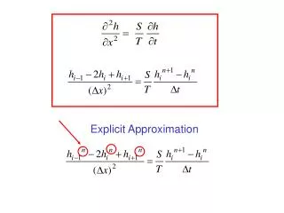
Explicit Approximation
Explicit Approximation. Explicit Solution. Eqn. 4.11 (W&A). Everything on the RHS of the equation is known. Solve explicitly for ; no iteration is needed. Explicit approximations are unstable unless small time steps are used. Problems with explicit solution:

Explicit Approximation
E N D
Presentation Transcript
Explicit Solution Eqn. 4.11 (W&A) Everything on the RHS of the equation is known. Solve explicitly for ; no iteration is needed. Explicit approximations are unstable unless small time steps are used.
Problems with explicit solution: • Requires small time step • Unnatural propagation of boundary effect • Large mass balance error for some time steps suggests • t = 5 minutes is too large.
In general: where = 1 for fully implicit = 0.5 for Crank-Nicolson = 0 for explicit
Implicit Solution and use Gauss-Seidel iteration. Solve for
n+1 t m+3 Iteration planes m+2 m+1 n
Implicit Solution Spreadsheet
t = 5 Note: at t=5 min, the boundary effect is propagated past the first node near the boundary.
Computational molecules Implicit solution Explicit solution
t = 10 Compare with matrix solution given in directions for Problem Set 3.
t = 5 Note: at t=5 min, the boundary effect is propagated past the first node near the boundary.
Sensitivity to time step at x = 90 m t = 5 minutes t = 10 minutes
Use of a time step multiplier Most transient problems will “shock” the system at the beginning of the simulation. The shock could be a drop in water level or the start of pumping, for example. The system will respond rapidly to the “shock” and to capture this rapid response it is necessary to use small time steps. Such small time steps are not necessary later in the simulation. Hence, a time step multiplier increases the size of the time step as the solution progresses.
Use of a time step multiplier tnew = told x MULT where MULT is the time step multiplier, e.g., 1.2
Could also solve the implicit finite difference equation using SOR iteration. Gauss-Seidel value
Another option for solving the implicit finite difference eqn. is a “direct solution” using matrix methods. All known terms are on the RHS; all unknown terms are on the LHS. Solve this equation using matrix methods. See W&A, p. 95