Chapter (7) The relational Data Model, Relational Constraints, and the Relational Algebra

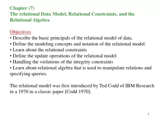
1. Chapter (7) • The relational Data Model, Relational Constraints, and the Relational Algebra • Objectives • Describe the basic principals of the relational model of data. • Define the modeling concepts and notation of the relational model. • Learn about the relational constraints • Define the update operations of the relational model • Handling the violations of the integrity constraints • Learn about relational algebra that is used to manipulate relations and specifying queries. • The relational model was first introduced by Ted Codd of IBM Research in a 1970 in a classic paper [Codd 1970].

2. Relational Model Concepts The relational model represents the database as a collection of relations. A relation is often resembles a table of values or to some extent, a “flat” file of records. There are important differences between relations and files. A relation that is thought as a table of values contains rows that represent a collection of related values. In the formal relational model terminology, a row is called a tuple, a column header is called an attribute, and the table is called a relation. The data type describing the types of values that can appear in each column is called a domain.

3. Domains A domain D is a set of values that are indivisible as far as the relational model is concerned, i.e., it contains of a set of atomic values. Examples: USA_Phone numbers. Which is ….. Local_phone_numbers. Which is … Names: The set of names of persons. Social_security_numbers: The set of valid 9-digit social security numbers. GPA: A real value between 0 and 4. There is a data type of format associated with each domain. Relation A relation schemaR, denoted by R(A1, A2, …, An) is made up of a relation name R and a list of attributes A1, A2, …, An. Each attribute Ai is the name of a role played by some domain D in the relation schema R. D is called the domain of Ai and is denoted by Dom(Ai).

4. Relation-cont. • A relation schema is used to describe a relation, R is called the name of this relation. • The degree of a relation is the number of attributes n of its relation schema. What are the domains?

5. Relation-cont. • A relation r(R) is a mathematical relation of degree n on the domains dom(A1), dom(A2), …, dom(An). If we denote number of values or cardinality of a domain D by |D|, and assume that all domains are finite, the total number of tuples in the above Cartesian product is: This represents many combinations, out of which, a relation state at a given time – the current relation state – reflects only the valid tuples that represent a particular state of the real world. It is possible that several attributes have the same domain. The attributes indicate different roles, or interpretations, for the domain.

6. Characteristics of Relations There are several characteristics that separate a table from a relation: 1. Ordering of Tuples in a Relation The records in a file are in some order, 1st, 2nd, … ith. While in a relation, such ordering does not exist. Tuple ordering is not part of relation definition. 2. Ordering of Values within a Tuple, and an Alternative Definition of a Relation. The ordering of values (attributes) in a relation schema definition is important. However, at the logical level, the order of attributes and there their values are not really important as long as the correspondence between attributes and values is maintained. In an alternative definition can be given such that the ordering of tuples in a relation is not necessary.

7. 2. Ordering of Values within a Tuple, and an Alternative Definition ofa Relation. – cont. In this definition, t[Ai] must be in dom(Ai) for for each mapping t in r. According to this definition, a tuple can be considered as a set of (<attributes>, <value>) pairs, where each pair gives the value of the mapping from an attribute Ai to a value vi from dom(Ai).

8. 3. Values in the Tuples Each value is a tuple is an atomic value, i.e., is not divisible into components within the framework of the basic relational model. Composite and multivalued attributes are not allowed. Multivalued attributes must be represented by separate relations, and composite attributes are represented only by their simple component attributes. The values of some attributes within a particular tuple may be unknown or may not apply to that tuple. For such cases a value called null is used. A null value may have one the following values: “value unknown”, value exists but not available”, or “attribute does not apply to this tuple.” Incorporating different types of null values into relational model operations has proved difficult.

9. 4. Interpretation of a Relation The relation schema can be interpreted as a declaration or a type of assertion. Example: In relation STUDENT (Fig. 7.1) each tuple contains the: Name, SSN, HomePhone, Address, OfficePhone, Age, and GPA. Thus, each tuple is reflecting a fact or a particular instance of assertion. Some relations may represents facts about entities, whereas other relations may represent facts about relationships. Example: A relation schema MAJORS (StudentSSN, DepartmentCode) asserts that students major in academic departments. A tuple in this relation relates a student to his or her major department. Hence, the relational model represents facts about both entities and relationships uniformly as relations.

10. Relational Model Notation • Following notation is commonly used: • A relation schema R of degree n is denoted by R(A1, A2,…,An). • An n-tuple t in a relation r(R) is denoted by t = <v1, v2, …, vn>, where vi is the value corresponding to attribute Ai. The components values of tuples are denoted as: • Both t[Ai] and t.Ai refer to the value vi in t for attribute Ai. • Both t[Au, Aw, …,Az] and t.(Au, Aw, …,Az), where Au, Aw, …,Az is a list of all attributes from R, refer to the subtuple of values < v1, v2, …, vn> from t corresponding to the attributes specified in the list. • The letters Q, R, S denote relation names. • The letters q, r, s denote relation states • The letters t, u, v denote tuples • The name of a relation schema also refers to the current set of tuples in that relation. • An attribute A can be qualified with the relation name R to which it belongs by using the dot notation R.A. STUDENT.Name, EMPLOYEE.Name.

11. Relational Constraints and Relational Database Schemas We will discuss various constraints on data that can be specified on a relational database schema in the form of constraints. Common constraints are: Domain constraints Key constraints Entity integrity Referential integrity Other types of constraints are: Data dependencies (functional and multivalued) Which is used mainly for design and is is discussed in Chapter 14 and 15.

12. Domain Constraints The value of each attribute A must be an atomic value from the domain dom(A). The data types associated with domains typically include standard numeric data types for: integers (short-integer, integer, long-integer) real numbers (float and double-precision float) Characters, fixed-length strings, and variable length strings are also available. Others possibilities: Date, Time, Timestamp, and Money data types.

13. Key Constraints A relation is a set of tuples. By definition, all elements of a set are distinct, hence, all tuples in a relation must also be distinct. Suppose we denote a subset of relation R as SK such that no two tuples in any relation r of R have the same combination of values for these attributes. Then, for any two distinct tuples t1 and t2 in a relation state r of R, we have the constraint that: Any such set of attributes SK is called a superkey of the relation schema R. The superkey specifies a uniqueness constraint that no two distinct tuples in state r of R can have the same value for SK.

14. Key Constraints – cont. Every relation has at least one default superkey (the set of all its attributes). A superkey can have redundant attributes, however, no redundancy no redundancy is desirable. A key (K) of a relation schema R is a superkey of R with the additional property that removing any attribute A from K leaves a set of attributes K’ that is not a superkey of R. Example: Set[SSN] is a key of STUDENT relation. No two students can have the same SSN, thus any set of attributes {SSN, Name, Age} or {SSN, Name, Class} is a superkey. But, neither one of these are the key to STUDENT, because removing Name, Age, or both still leaves the remaining a superkey.

15. Key Constraints – cont. A key is time-invariant, which means, once defined at the stage 0, it cannot be changed at the later stage of the relation. If a relation schema has more than one key each of the keys is called a candidate key. One of the candidate keys can be defined as the primary key. Example: CAR LicenseNumber EngineSerialNumber Make Model Year Both LicenseNumber and EngineSerialNumber are keys. Either one of these two can be defined as the primary key for that relation. It is better to choose a primary key with a single attribute or small number of attributes. Can you give an example?

16. Relational Databases and Relational Database Schemas In general a relational database schema S is a set of relation schemas S = {R1, R2, …, Rm} and a set of integrity constraints (IC). A relational database state DB of S is a set of relation states DB = {r1, r2, …, rm} Such that each ri is a state of Ri and such that the ri relation states satisfy the integrity constraints specified in IC. Think about the COMPANY relational database schema: COMPANY = {EMPLOYEE, DEPARTMENT, DEPT_LOCATION, PROJECT, WORKS_ON, DEPENDENT} Each relational DBMS must have a Data Definition Language (DDL) for defining a relational database schema. Current DBMSs are mostly using SQL.

17. Integrity, Referential Integrity, and Foreign Keys The entity integrity constraint states that no primary key can be null. Why? The referential integrity constraint is specified between two relations and is used to maintain the consistency among tuples of two relations. You must refer to an existing tuple at all time. There is another type of constraint called semantic integrity constraints. Examples of this type of constraints is the salary of an employee that must be less than that of his/her supervisor. Or maximum number of hours that an employee can work which must be less than 56 hours/week. These types of constraints can be specified and enforced using a general purpose constraints specification language. A mechanism called triggers and assertions can be used.

18. Integrity, Referential Integrity, and Foreign Keys – cont. The previous constraints also are known as state constraints, because they define the constraints that a valid state of the database must satisfy. Another type of constraint is called transition constraint. This constraint deals with the changes in the database. An example is the salary of employees that can only increase. The four types of constraints are: Domain Constraints Key Constraints and Constraints on null Entity Integrity Referential Integrity

19. Update Operations and Dealing with Constraint Violations The main operations of the relational model can be categorized into retrieval and updates. There are three basic update operations: Insert is used to insert new tuple or tuples in a relation. Delete is used to delete tuples. Modify is used to change the values of some attributes in existing tuples. Whenever an update operation is applied, the integrity constraints specified on the relational database schema should not be violated.

20. A Quick Note The insertion, deletion, and update is only possible when the table (entity) which is the target of these modifications already exists. In Chapter (8) we will discuss the creation of tables. Just to give you an idea how the CREATE command looks like, I have listed the CREATE procedure for EMPLOYEE table below. CREATE TABLE EMPLOYEE (FNAME VARCHAR(15) NOT NULL, MINIT CHAR, LNAME VARCHAR(15) NOT NULL, SSN CHAR(9) NOT NULL, BDATE DATE, ADDRESS VARCHAR(30), SEX CHAR, SALARY DECIMAL(10,2), SUPERSSN CHAR(9), DNO INT NOT NULL, PRIMARY KEY (SSN), FOREIGN KEY (SUPPERSSN) REFERENCES EMPLOYEE(SSN), FOREIGN KEY (DNO) REFERENCES DEPARTMENT (DNUMBER);

21. The Insert Operations • The insert operation provides a list of values for a new tuple t that is to be inserted into a relation R. • Insert can violate any of the four constraints that we discussed earlier. • Domain constraint can be violated if an attribute value is given that does not appear in the corresponding domain. • Insert <‘Cecilia’, ‘F’, ‘Kolonsky’, null, ‘1960-04-05’,’6357 Windy Lane, Katy, TX’, F, 28000, null, 4 > into EMPLOYEE. • What is violated here? • Key constraint can be violated if a key value in the new tuple t already exists in another tuple in the relation r(R). • Insert<‘Alicia’, ‘J’, ‘Zelaya’, ‘999887777’,’1960-04-05’,’6357 Windy Lane, Katy, TX’, F, 28000, ‘987654321’,4 > into EMPLOYEE. • What is violated here?

22. The Insert Operation – cont. • Entity integrity can be violated if reference is made to an invalid attribute. • Insert <‘Cecilia’, ‘F’, ‘Kolonsky’, ‘677678989’, ‘1960-04-05’,’6357 Windswept, Katy, TX’, F, 28000, ‘987654321’, 7 > into EMPLOYEE. • What is violated here? • Referential integrity can be violated if the value of any foreign key in t refers to a tuple that does not exist in the referenced relation. • Insert <‘Cecilia’, ‘F’, ‘Kolonsky’, ‘677678989’, ‘1960-04-05’,’6357 Windy Lane, Katy, TX’, F, 28000, null, 4 > into EMPLOYEE. • What is violated here?

23. The Insert Operation – cont. If an insertion violates any of the four constraints, it will be rejected. In case of rejection, it would be useful if the DBMS could explain to the user why the insertion was rejected. Another option is to attempt to correct the problem. This is not common for Insert rather for Delete and Update. Example: In operation (1) in the previous page, the DBMS could ask user to provide a value for SSN and accept the insertion if a valid SSN value were provided.

24. The Delete Operation The Delete operation can violate only referential integrity, if the tuple being deleted is referenced by the foreign keys from other tuples in the database. Examples: 1. Delete the WORKS_ON tuple with ESSN = ‘999887777’ and PNO = 10. Is this deletion accepted? 2. Delete the EMPLOYEE tuple with SSN=‘999887777’. How about this one? 3. Delete the EMPLOYEE tuple with SSN=‘333445555’, What kind of problem this deletion will cause? Three options are available: 1) reject the deletion 2) attempt to cascade (propagate) the deletion to to the references 3) modify the the referencing attribute values that cause the violation (set to null or changed to reference to another valid tuple).

25. The Update Operation • The Update is used to change the values of one or more attributes in a tuple (or tuples) of some relation R. • Examples: • Update the SALARY of the EMPLOYEE tuple with SSN = ‘999887777’ to 28000. • Will this be accepted? • 2. Update the DNO of the EMPLOYEE tuple with SSN=‘999887777’ to 1. • Will this be accepted? • 3. Update the DNO of the EMPOYEE tuple with SSN=‘999887777’ to 7. • Will this be accepted? • 4. Update the SSN of the EMPLOYEE tuple with SSN=‘999887777’ to ‘987654321’. • Will this be accepted?

26. Basic Relational Algebra Operations • A data model must include a set of operations to manipulate the data. • A basic set of relational model operations constitute the relational algebra. • These operations enable the user to specify basic retrieval requests. • The result of a retrieval is a new relation, which may have been formed from one or more relations. • A sequence of relational algebra operations forms a relational algebra expression, whose result will also be a relation. • The relational algebra operations are two types: • 1) set operations from mathematical set theory (UNION, INTERSECTION, SET DIFFERENCE, and CARTESIAN PRODUCT). • 2) operations developed specifically for relational databases (SELECT, PROJECT, and JOIN, etc…).

27. The SELECT Operation The SELECT operation is used to select a subset of the tuples from a relation that satisfy a selection condition. The SELECT operation works like a filter that allows the tuples, which satisfy a specific qualification to pass through. Example: Select from EMPLOYEE those who work in DNO = 4 Select from EMPLOYEE those with Salary > 30,000 ……… The general form of SELECT is:

28. The SELECT Operation – cont. • The selection condition is a Boolean expression and R is generally a relational algebra expression which will result in a relation. • The relation resulting from the SELECT operation has the same attributes as R. • The Boolean expression may have one the following forms: • <attribute name> <comparison op> <constant value> OR • <attribute name> <comparison op> <attribute name> • attribute name: the name of an attribute R • comparison op: one of the operators; • Note: If the domains of the attributes are not ordered values (numeric or date) then we only can use . An example is Color={red, blue, green, …}.

29. The SELECT Operation – cont. The SELECTION process: The selection condition is applied independently to each tuple t in R (substitute each occurrence of an attribute Ai in the selection condition with its value in the tuple t[Ai]. If the condition evaluates to true, the tuple is selected. Choices for Boolean operations are; AND, OR, and NOT. Can you determine under what conditions these are true or false? The SELECT operator is unary (can be applied to only a single relation). In addition, the selection operation is applied to each tuple individually. The SELECT operation is commutative:

30. The SELECT Operation – cont. We can also combine a cascade of SELECT operations into a single SELECT operation with conjunctive (AND) condition: Example: Select Senior Students, majoring in CS, with GPA higher than 3.0, who are from NC.

31. The PROJECT Operation The SELECT operation selects some of the rows from the table while discarding other rows. The PROJECT operation, on the other hand, selects certain columns from the table and discards the other columns. Example: To list each employee’s first and last name and salary, we can use the PROJECT operation as follows: General form:

32. The PROJECT Operation – cont. If the attribute list includes only nonkey attributes of R, duplicate are likely to occur. The PROJECT operation removes any duplicate tuples. This is known as duplicate elimination. Example: The result is shown on the previous page in Table (c). The tuple <F,25000> appears only once. The number of tuples in a relation resulting from a PROJECT operation is always less than or equal to the number of tuples in R. If the projection list is a superkey of R – that is, it includes some key of R – the resulting relation has the same number of attributes. Is this always true? This is true as long as <list2> contains the attributes in <list1>. Note: commutativity DOES NOT hold on PROJECT.

33. Sequence of Operations and the RENAME Operation Sometimes we apply several relational algebra operations one after the other. In such cases we have two choices: - write the operations as a single relational algebra expression by nesting the operations, or - apply one operation at a time and create intermediate result relations. In the later case, we must name the relations that hold the intermediate results. Example: list First name, Last name, and salary of all employees who work in department number 5. How do we do this? SELECT all employees in department 5, then PROJECT their First name, Last name and Salaries.

35. Sequence of Operations and the RENAME Operation – cont. We can show the sequence of operations, giving a name to each intermediate relation: We can also use this technique to rename the attributes in the intermediate and result relations. See Figure 9.b.

36. The RENAME Operation • The general format of the RENAME operation is: • To rename both the relation and its attributes we will use: • To rename the relation only: • To rename the attributes only:

37. Set Theoretic Operations These are the set of standard mathematical operations. Example:Retrieve the SSN of all employees who either work in department 5 OR directly supervise an employee who works in department 5. Two relations participating in a UNION must be union compatible, i.e., the have the same degree and their domains are the same.

38. Set Theoretic Operations – cont. • Other theoretic operators are: • UNION, INTERSECTION, and SET DIFFERENCE. These are all binary operators. They are defines as: • UNION: The result of this operation, denoted by R D S, is a relation that includes all tuples that are either in R or in S or in both R and S. Duplicate tuples are eliminated. • INTERSECTION: The result of this operation, denoted by R C S, is a relation that includes all tuples that are in both R and S. • SET DIFFERENCE: The result of this operation, denoted by R - S, is a relation that includes all tuples that are in R but not in S. • The UNION and INTERSECTION are commutative operations. That is: • Example: List the First name and Last name of those who are either a student or an employee. Fig. 11.b. • List those who are both student and instructor. Fig. 11.c.

39. Figure 11.

40. Set Theoretic Operations – cont. Both union and intersection can be treated as n-ray operations applicable to any number of relations as both are associative operations; that is: The DIFFERENCE operation is not commutative; that is, List the name of students who are not instructors. Fig. 11.d. What is shown on Fig. 11.e?

41. The CARTESIAN PRODUCT Operation (CROSS PRODUCT or CROSS JOIN) This is denoted by X, which is also a binary set operation, but the relations on which it is applied do not have to be union compatible. In general, we have: R(A1, A2, …,An) X S(B1, B2, …,Bm) = Q(A1, A2, …,An,B1, B2, …,Bm) Where, Q with n+m attributes in the order shown above. Example: For each female employee, list the names of her dependents:

44. The JOIN Operations The join operation is denoted by , is used to combine related tuples from two relations into single tuples. Example: List the managers of all departments. What do we need to do to get this? In previous example: We can can keep these two And replace these two with

45. The JOIN Operations – cont. The general form of JOIN operations is: This will result in a relation Q with n+m attributes. What is the difference between CARTESIAN PRODUCT and JOIN? JOIN: will combine all tuples that satisfy the join condition. CARTESIAN PRODUCT: will combine all tuples. A general join condition is of the form: <condition> AND <condition> AND …<condition> Where each condition is of the form Ai Bj, Ai is an attribute of R, Bj is an attribute of S, Ai and Bj have the same domain, and refers to one of the operations: . A JOIN operation with such a general join condition is called a THETA JOIN.

46. The JOIN Operations – cont. The most common JOIN involves join condition with equality comparisons only. Such a JOIN is called EQUIJOIN. What do you observer in Figure 7.13 (MGSSN & SSN)? In order to avoid repetition of same entities we use NATURAL JOIN which is denoted by *. The standard definition of NATURAL JOIN requires that the two join attributes (or each pair of join attributes) have the same name in both relations. If that is not the case, the renaming operation is applied first: In the above example, the attribute DNUM is called the join attribute.

47. The JOIN Operations – cont. Example: PROJ_DEPT PNAME PNUMBER PLOCATION DNUM DNAME MGRSS MGRSTARTDATE DEPT_LOCS DNAME DNUMBER MGRSSN MGRSTARTDATE LOCATION How many ways can we JOIN the above relations? The more general but not standard definition for NATURAL-JOIN is: What if there is nothing that can be joined? A JOIN operation can be used in combination. What does the following do?

48. A Complete Set of Relational Algebra Operations It has been shown that the set of relational algebra operations is complete set. What does it mean? It means that any of the other relational algebra operations can be expressed as a sequence of operations from this set. Example: This how the INTERSECTION operation is represented in terms of others. Show the JOIN operation in terms of CARTESIAN PRODUCT and SELECT.